Page 297 -

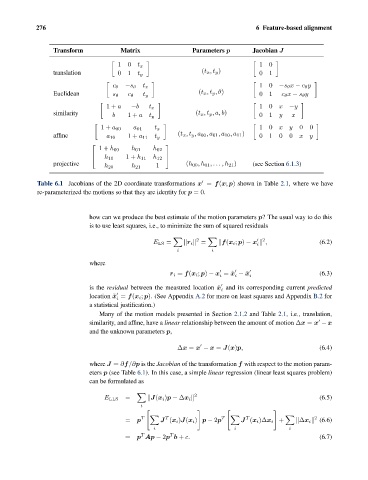
276 6 Feature-based alignment

Transform Matrix Parameters p Jacobian J

10 t x 10
translation 01 t y (t x ,t y ) 01

c θ −s θ t x 10 −s θ x − c θ y
Euclidean s θ c θ t y (t x ,t y ,θ) 01 c θ x − s θ y

1+ a −b t x 10 x −y
similarity b 1+ a t y (t x ,t y ,a,b) 01 y x

10 xy 0 0
1+ a 00 a 01 t x
affine a 10 1+ a 11 t y (t x ,t y ,a 00 ,a 01 ,a 10 ,a 11 ) 01 0 0 xy
⎡ ⎤
1+ h 00 h 01 h 02
h 10 1+ h 11 h 12
⎣ ⎦
projective (h 00 ,h 01 ,...,h 21 ) (see Section 6.1.3)
h 20 h 21 1
Table 6.1 Jacobians of the 2D coordinate transformations x = f(x; p) shown in Table 2.1, where we have

re-parameterized the motions so that they are identity for p =0.

how can we produce the best estimate of the motion parameters p? The usual way to do this
is to use least squares, i.e., to minimize the sum of squared residuals

2 2
E LS = r i = f(x i ; p) − x , (6.2)
i
i i
where

r i = f(x i ; p) − x = ˆ x − ˜ x i (6.3)
i
i
is the residual between the measured location ˆ x and its corresponding current predicted

i
location ˜ x = f(x i ; p). (See Appendix A.2 for more on least squares and Appendix B.2 for

i
a statistical justification.)
Many of the motion models presented in Section 2.1.2 and Table 2.1, i.e., translation,
similarity, and affine, have a linear relationship between the amount of motion Δx = x − x

and the unknown parameters p,
Δx = x − x = J(x)p, (6.4)

where J = ∂f/∂p is the Jacobian of the transformation f with respect to the motion param-
eters p (see Table 6.1). In this case, a simple linear regression (linear least squares problem)
can be formulated as

2
= (6.5)
E LLS J(x i )p − Δx i
i

T T T T 2
= p J (x i )J(x i ) p − 2p J (x i )Δx i + Δx i (6.6)
i i i
T
T
= p Ap − 2p b + c. (6.7)