Page 301 -

280 6 Feature-based alignment

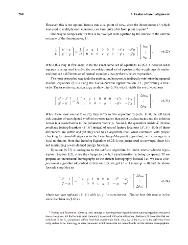
However, this is not optimal from a statistical point of view, since the denominator D, which
was used to multiply each equation, can vary quite a bit from point to point. 6
One way to compensate for this is to reweight each equation by the inverse of the current
estimate of the denominator, D,

⎡ ⎤
h 00

1 ˆ x − x 1 xy 1 0 0 0 −ˆx x −ˆx y .

= ⎢ . ⎦ . (6.22)
⎥

D ˆ y − y D 0 0 0 xy 1 −ˆy x −ˆy y ⎣ .

h 21
While this may at first seem to be the exact same set of equations as (6.21), because least
squares is being used to solve the over-determined set of equations, the weightings do matter
and produce a different set of normal equations that performs better in practice.
The most principled way to do the estimation, however, is to directly minimize the squared
residual equations (6.13) using the Gauss–Newton approximation, i.e., performing a first-
order Taylor series expansion in p, as shown in (6.14), which yields the set of equations
⎡ ⎤
Δh 00
ˆ x − ˜x 1 xy 1 0 0 0 −˜x x −˜x y .

= ⎢ . ⎦ . (6.23)
⎥
ˆ y − ˜y D 0 0 0 xy 1 −˜y x −˜y y ⎣ .

Δh 21
While these look similar to (6.22), they differ in two important respects. First, the left hand
side consists of unweighted prediction errors rather than point displacements and the solution
vector is a perturbation to the parameter vector p. Second, the quantities inside J involve

predicted feature locations (˜x , ˜y ) instead of sensed feature locations (ˆx , ˆy ). Both of these
differences are subtle and yet they lead to an algorithm that, when combined with proper
checking for downhill steps (as in the Levenberg–Marquardt algorithm), will converge to a
local minimum. Note that iterating Equations (6.22) is not guaranteed to converge, since it is
not minimizing a well-defined energy function.
Equation (6.23) is analogous to the additive algorithm for direct intensity-based regis-
tration (Section 8.2), since the change to the full transformation is being computed. If we
prepend an incremental homography to the current homography instead, i.e., we use a com-
positional algorithm (described in Section 8.2), we get D =1 (since p =0) and the above
formula simplifies to
⎡ ⎤
Δh 00
2

ˆ x − x xy 1 0 0 0 −x −xy .
= ⎢ . . ⎦ , (6.24)
⎥

ˆ y − y 0 0 0 xy 1 −xy −y 2 ⎣
Δh 21
where we have replaced (˜x , ˜y ) with (x, y) for conciseness. (Notice how this results in the

same Jacobian as (8.63).)
6 Hartley and Zisserman (2004) call this strategy of forming linear equations from rational equations the direct
linear transform, but that term is more commonly associated with pose estimation (Section 6.2). Note also that our
definition of the h ij parameters differs from that used in their book, since we define h ii to be the difference from
unity and we do not leave h 22 as a free parameter, which means that we cannot handle certain extreme homographies.