Page 303 -

282 6 Feature-based alignment

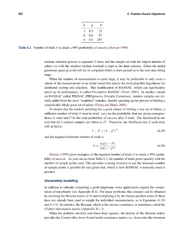
k p S
3 0.5 35
6 0.6 97
6 0.5 293

Table 6.2 Number of trials S to attain a 99% probability of success (Stewart 1999).

random selection process is repeated S times and the sample set with the largest number of
inliers (or with the smallest median residual) is kept as the final solution. Either the initial
parameter guess p or the full set of computed inliers is then passed on to the next data fitting
stage.
When the number of measurements is quite large, it may be preferable to only score a
subset of the measurements in an initial round that selects the most plausible hypotheses for
additional scoring and selection. This modification of RANSAC, which can significantly
speed up its performance, is called Preemptive RANSAC (Nist´ er 2003). In another variant
on RANSAC called PROSAC (PROgressive SAmple Consensus), random samples are ini-
tially added from the most “confident” matches, thereby speeding up the process of finding a
(statistically) likely good set of inliers (Chum and Matas 2005).
To ensure that the random sampling has a good chance of finding a true set of inliers, a
sufficient number of trials S must be tried. Let p be the probability that any given correspon-
dence is valid and P be the total probability of success after S trials. The likelihood in one
k
trial that all k random samples are inliers is p . Therefore, the likelihood that S such trials
will all fail is
k S
1 − P =(1 − p ) (6.29)
and the required minimum number of trials is
log(1 − P)
S = . (6.30)
k
log(1 − p )
Stewart (1999) gives examples of the required number of trials S to attain a 99% proba-
bility of success. As you can see from Table 6.2, the number of trials grows quickly with the
number of sample points used. This provides a strong incentive to use the minimum number
of sample points k possible for any given trial, which is how RANSAC is normally used in
practice.

Uncertainty modeling
In addition to robustly computing a good alignment, some applications require the compu-
tation of uncertainty (see Appendix B.6). For linear problems, this estimate can be obtained
by inverting the Hessian matrix (6.9) and multiplying it by the feature position noise (if these
have not already been used to weight the individual measurements, as in Equations (6.10)
and 6.11)). In statistics, the Hessian, which is the inverse covariance, is sometimes called the
(Fisher) information matrix (Appendix B.1.1).
When the problem involves non-linear least squares, the inverse of the Hessian matrix
provides the Cramer–Rao lower bound on the covariance matrix, i.e., it provides the minimum