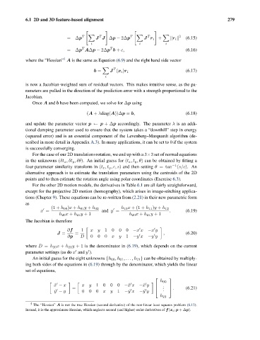
Page 300 -

6.1 2D and 3D feature-based alignment 279

T T T T 2
=Δp J J Δp − 2Δp J r i + r i (6.15)
i i i
T
T
=Δp AΔp − 2Δp b + c, (6.16)
5
where the “Hessian” A is the same as Equation (6.9) and the right hand side vector
T
b = J (x i )r i (6.17)
i
is now a Jacobian-weighted sum of residual vectors. This makes intuitive sense, as the pa-
rameters are pulled in the direction of the prediction error with a strength proportional to the
Jacobian.
Once A and b have been computed, we solve for Δp using
(A + λdiag(A))Δp = b, (6.18)

and update the parameter vector p ← p +Δp accordingly. The parameter λ is an addi-
tional damping parameter used to ensure that the system takes a “downhill” step in energy
(squared error) and is an essential component of the Levenberg–Marquardt algorithm (de-
scribed in more detail in Appendix A.3). In many applications, it can be set to 0 if the system
is successfully converging.
For the case of our 2D translation+rotation, we end up with a 3×3 set of normal equations
in the unknowns (δt x ,δt y ,δθ). An initial guess for (t x ,t y ,θ) can be obtained by fitting a
four-parameter similarity transform in (t x ,t y ,c,s) and then setting θ = tan −1 (s/c).An
alternative approach is to estimate the translation parameters using the centroids of the 2D
points and to then estimate the rotation angle using polar coordinates (Exercise 6.3).
For the other 2D motion models, the derivatives in Table 6.1 are all fairly straightforward,
except for the projective 2D motion (homography), which arises in image-stitching applica-
tions (Chapter 9). These equations can be re-written from (2.21) in their new parametric form
as
(1 + h 00 )x + h 01 y + h 02 h 10 x +(1+ h 11 )y + h 12
x = and y = . (6.19)

h 20 x + h 21 y +1 h 20 x + h 21 y +1
The Jacobian is therefore

∂f 1 xy 1 0 0 0 −x x −x y

J = = , (6.20)

∂p D 0 0 0 xy 1 −y x −y y
where D = h 20 x + h 21 y +1 is the denominator in (6.19), which depends on the current

parameter settings (as do x and y ).

An initial guess for the eight unknowns {h 00 ,h 01 ,...,h 21 } can be obtained by multiply-
ing both sides of the equations in (6.19) through by the denominator, which yields the linear
set of equations,
⎡ ⎤
h 00
ˆ x − x xy 1 0 0 0 −ˆx x −ˆx y .

= ⎢ . ⎦ . (6.21)
⎥
ˆ y − y 0 0 0 xy 1 −ˆy x −ˆy y ⎣ .

h 21
5 The “Hessian” A is not the true Hessian (second derivative) of the non-linear least squares problem (6.13).
Instead, it is the approximate Hessian, which neglects second (and higher) order derivatives of f(x i ; p +Δp).