Page 299 -

278 6 Feature-based alignment

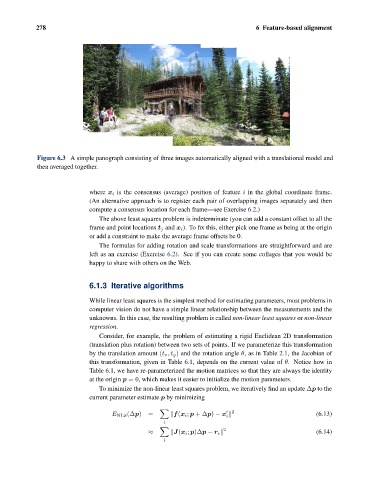
Figure 6.3 A simple panograph consisting of three images automatically aligned with a translational model and
then averaged together.

where x i is the consensus (average) position of feature i in the global coordinate frame.
(An alternative approach is to register each pair of overlapping images separately and then
compute a consensus location for each frame—see Exercise 6.2.)
The above least squares problem is indeterminate (you can add a constant offset to all the
frame and point locations t j and x i ). To fix this, either pick one frame as being at the origin
or add a constraint to make the average frame offsets be 0.
The formulas for adding rotation and scale transformations are straightforward and are
left as an exercise (Exercise 6.2). See if you can create some collages that you would be
happy to share with others on the Web.

6.1.3 Iterative algorithms

While linear least squares is the simplest method for estimating parameters, most problems in
computer vision do not have a simple linear relationship between the measurements and the
unknowns. In this case, the resulting problem is called non-linear least squares or non-linear
regression.
Consider, for example, the problem of estimating a rigid Euclidean 2D transformation
(translation plus rotation) between two sets of points. If we parameterize this transformation
by the translation amount (t x ,t y ) and the rotation angle θ, as in Table 2.1, the Jacobian of
this transformation, given in Table 6.1, depends on the current value of θ. Notice how in
Table 6.1, we have re-parameterized the motion matrices so that they are always the identity
at the origin p =0, which makes it easier to initialize the motion parameters.
To minimize the non-linear least squares problem, we iteratively find an update Δp to the
current parameter estimate p by minimizing

2
E NLS (Δp)= f(x i ; p +Δp) − x (6.13)
i
i
2

≈ J(x i ; p)Δp − r i (6.14)
i