Page 306 -

6.2 Pose estimation 285

p i = (X i,Y i,Z i,W i)

d i
d ij

x i
p j
ș ij d j
c x j

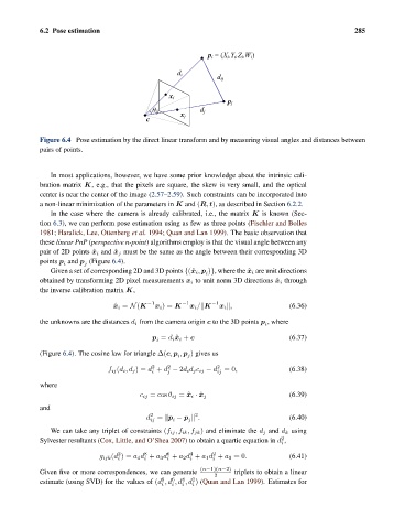
Figure 6.4 Pose estimation by the direct linear transform and by measuring visual angles and distances between
pairs of points.

In most applications, however, we have some prior knowledge about the intrinsic cali-
bration matrix K, e.g., that the pixels are square, the skew is very small, and the optical
center is near the center of the image (2.57–2.59). Such constraints can be incorporated into
a non-linear minimization of the parameters in K and (R, t), as described in Section 6.2.2.
In the case where the camera is already calibrated, i.e., the matrix K is known (Sec-
tion 6.3), we can perform pose estimation using as few as three points (Fischler and Bolles
1981; Haralick, Lee, Ottenberg et al. 1994; Quan and Lan 1999). The basic observation that
these linear PnP (perspective n-point) algorithms employ is that the visual angle between any
pair of 2D points ˆ x i and ˆ x j must be the same as the angle between their corresponding 3D
points p and p (Figure 6.4).
i
j
Given a set of corresponding 2D and 3D points {(ˆ x i , p )}, where the ˆ x i are unit directions
i
obtained by transforming 2D pixel measurements x i to unit norm 3D directions ˆ x i through
the inverse calibration matrix K,
ˆ x i = N(K −1 x i )= K −1 x i / K −1 x i , (6.36)

the unknowns are the distances d i from the camera origin c to the 3D points p , where
i
p = d i ˆ x i + c (6.37)
i
(Figure 6.4). The cosine law for triangle Δ(c, p , p ) gives us
i j
2
2
2
f ij (d i ,d j )= d + d − 2d i d j c ij − d =0, (6.38)
i j ij
where
(6.39)
c ij = cos θ ij = ˆ x i · ˆ x j
and
2
2
d = p − p . (6.40)
ij
i
j
We can take any triplet of constraints (f ij ,f ik ,f jk ) and eliminate the d j and d k using
2
Sylvester resultants (Cox, Little, and O’Shea 2007) to obtain a quartic equation in d ,
i
8
4
2
6
2
g ijk (d )= a 4 d + a 3 d + a 2 d + a 1 d + a 0 =0. (6.41)
i
i
i
i
i
(n−1)(n−2)
Given five or more correspondences, we can generate triplets to obtain a linear
2
6
8
4
2
estimate (using SVD) for the values of (d ,d ,d ,d ) (Quan and Lan 1999). Estimates for
i i i i