Page 90 -

2.3 The digital camera 69

* =

f = 3/4 f = 5/4

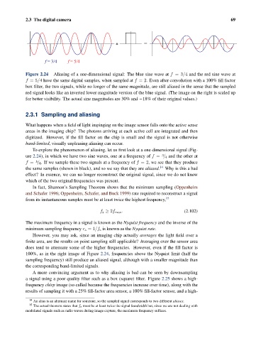
Figure 2.24 Aliasing of a one-dimensional signal: The blue sine wave at f =3/4 and the red sine wave at
f =5/4 have the same digital samples, when sampled at f =2. Even after convolution with a 100% fill factor
box filter, the two signals, while no longer of the same magnitude, are still aliased in the sense that the sampled
red signal looks like an inverted lower magnitude version of the blue signal. (The image on the right is scaled up
for better visibility. The actual sine magnitudes are 30% and −18% of their original values.)

2.3.1 Sampling and aliasing

What happens when a field of light impinging on the image sensor falls onto the active sense
areas in the imaging chip? The photons arriving at each active cell are integrated and then
digitized. However, if the fill factor on the chip is small and the signal is not otherwise
band-limited, visually unpleasing aliasing can occur.
To explore the phenomenon of aliasing, let us first look at a one-dimensional signal (Fig-
ure 2.24), in which we have two sine waves, one at a frequency of f = / 4 and the other at
3
5
f = / 4. If we sample these two signals at a frequency of f =2, we see that they produce
the same samples (shown in black), and so we say that they are aliased. 14 Why is this a bad
effect? In essence, we can no longer reconstruct the original signal, since we do not know
which of the two original frequencies was present.
In fact, Shannon’s Sampling Theorem shows that the minimum sampling (Oppenheim
and Schafer 1996; Oppenheim, Schafer, and Buck 1999) rate required to reconstruct a signal
from its instantaneous samples must be at least twice the highest frequency, 15

f s ≥ 2f max . (2.102)

The maximum frequency in a signal is known as the Nyquist frequency and the inverse of the
minimum sampling frequency r s =1/f s is known as the Nyquist rate.
However, you may ask, since an imaging chip actually averages the light field over a
finite area, are the results on point sampling still applicable? Averaging over the sensor area
does tend to attenuate some of the higher frequencies. However, even if the fill factor is
100%, as in the right image of Figure 2.24, frequencies above the Nyquist limit (half the
sampling frequency) still produce an aliased signal, although with a smaller magnitude than
the corresponding band-limited signals.
A more convincing argument as to why aliasing is bad can be seen by downsampling
a signal using a poor quality filter such as a box (square) filter. Figure 2.25 shows a high-
frequency chirp image (so called because the frequencies increase over time), along with the
results of sampling it with a 25% fill-factor area sensor, a 100% fill-factor sensor, and a high-
14 An alias is an alternate name for someone, so the sampled signal corresponds to two different aliases.
15 The actual theorem states that f s must be at least twice the signal bandwidth but, since we are not dealing with
modulated signals such as radio waves during image capture, the maximum frequency suffices.