Page 91 -

70 2 Image formation

(a) (b) (c) (d)

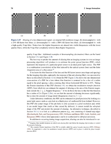
Figure 2.25 Aliasing of a two-dimensional signal: (a) original full-resolution image; (b) downsampled 4× with
a 25% fill factor box filter; (c) downsampled 4× with a 100% fill factor box filter; (d) downsampled 4× with
a high-quality 9-tap filter. Notice how the higher frequencies are aliased into visible frequencies with the lower
quality filters, while the 9-tap filter completely removes these higher frequencies.

quality 9-tap filter. Additional examples of downsampling (decimation) filters can be found
in Section 3.5.2 and Figure 3.30.
The best way to predict the amount of aliasing that an imaging system (or even an image
processing algorithm) will produce is to estimate the point spread function (PSF), which
represents the response of a particular pixel sensor to an ideal point light source. The PSF
is a combination (convolution) of the blur induced by the optical system (lens) and the finite
integration area of a chip sensor. 16
If we know the blur function of the lens and the fill factor (sensor area shape and spacing)
for the imaging chip (plus, optionally, the response of the anti-aliasing filter), we can convolve
these (as described in Section 3.2) to obtain the PSF. Figure 2.26a shows the one-dimensional
cross-section of a PSF for a lens whose blur function is assumed to be a disc of a radius
equal to the pixel spacing s plus a sensing chip whose horizontal fill factor is 80%. Taking
the Fourier transform of this PSF (Section 3.4), we obtain the modulation transfer function
(MTF), from which we can estimate the amount of aliasing as the area of the Fourier magni-
tude outside the f ≤ f s Nyquist frequency. 17 If we de-focus the lens so that the blur function
has a radius of 2s (Figure 2.26c), we see that the amount of aliasing decreases significantly,
but so does the amount of image detail (frequencies closer to f = f s ).
Under laboratory conditions, the PSF can be estimated (to pixel precision) by looking at a
point light source such as a pin hole in a black piece of cardboard lit from behind. However,
this PSF (the actual image of the pin hole) is only accurate to a pixel resolution and, while
it can model larger blur (such as blur caused by defocus), it cannot model the sub-pixel
shape of the PSF and predict the amount of aliasing. An alternative technique, described in
Section 10.1.4, is to look at a calibration pattern (e.g., one consisting of slanted step edges
(Reichenbach, Park, and Narayanswamy 1991; Williams and Burns 2001; Joshi, Szeliski, and
Kriegman 2008)) whose ideal appearance can be re-synthesized to sub-pixel precision.
In addition to occurring during image acquisition, aliasing can also be introduced in var-

16 Imaging chips usually interpose an optical anti-aliasing filter just before the imaging chip to reduce or control
the amount of aliasing.
17
The complex Fourier transform of the PSF is actually called the optical transfer function (OTF) (Williams
1999). Its magnitude is called the modulation transfer function (MTF) and its phase is called the phase transfer
function (PTF).