Page 520 - Corrosion Engineering Principles and Practice

486 C h a p t e r 1 2 C o r r o s i o n a s a R i s k 487

of the chemical inhibitor in the produced fluids. There may be applica-
tions where it is justified to apply a degree of over injection to provide
protection to downstream facilities where it is not practical to inject.
The KPI itself is derived from a measure of the produced fluids
including water and hydrocarbon phases and the inhibitor injected in
the produced fluid stream to provide a correlation between how
much inhibitor should be in the produced fluid stream versus actual
injected inhibitor concentrations. The KPI percent inhibitor availability
(Inhibitor ) function is described by Eq. (12.6):
AV
 C 
Inhibitor =  actual  × 100 (12.6)
AV C 
 required
where C actual is actual concentration of corrosion inhibitor (ppm) and
C is required concentration of corrosion inhibitor (ppm)
required
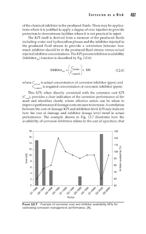
This KPI, when directly correlated with the corrosion cost KPI
(C corr ), provides a clear indication of the corrosion performance of the
asset and identifies clearly where effective action can be taken to
improve performance if damage costs are seen to increase. A correlation
between the cost of damage KPI and inhibition level KPI may indicate
how the cost of damage and inhibitor dosage level trend in actual
performance. The example shown in Fig. 12.7 illustrates how the
availability of corrosion inhibitors relates to the cost of operation, that

18 130
16 120
14
110
12
100
Cost (k$) 10 8 90 Inhibitor availability (%)

80
6
4 70
2 60
0 50
Q1-1998 Q2-1998 Q3-1998 Q4-1998 Q1-1999 Q2-1999 Q3-1999 Q4-1999 Q1-2000 Q2-2000 Q3-2000

Period
FIGURE 12.7 Example of corrosion cost and inhibitor availability KPIs for
estimating corrosion management performance. [8].