Page 103 - DSP Integrated Circuits

88 Chapter 3 Digital Signal Processing

Several variations of the Cooley—Tukey algorithm have since been derived.
These algorithms are collectively referred to as the FFT (fast Fourier transform).
Note that the FFT is not a new transform, it simply denotes a class of algorithms
for efficient computation of the discrete Fourier transform.
Originally, the aim in developing fast DFT algorithms was to reduce the num-
ber of fixed-point multiplications, since multiplication was more time consuming
and expensive than addition. As a by-product, the number of additions was also
reduced. This fact is important in implementations using signal processors with
floating-point arithmetic, since floating-point addition requires a slightly longer
time than multiplication.
Because of the high computational efficiency of the FFT algorithm, it is effi-
cient to implement long FIR filters by partitioning the input sequence into a set of
finite-length segments. The FIR filter is realized by successively computing the
DFT of an input segment and multiplying it by the DFT of the impulse response.
Next, an output segment is computed by taking the IDFT of the product. Finally,
the output segments are combined into a proper output sequence. Note that the
DFT of the impulse response needs to be computed only once. This method is com-
petitive with ordinary time domain realizations for FIR filters of lengths exceeding
50 to 100 [6, 9,10, 21].

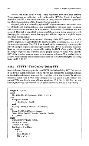
3.16.1 CT-FFT—The Cooley-Tukey FFT
Box 3.3 shows a Pascal program for the CT-FFT the Cooley-Tukey FFT. This version
of the FFT is called decimation-in-time FFT [9, 10], because the algorithm is based
on the divide-and-conquer approach that is applied in the time domain. We will only
discuss so-called radix-2 FFTs with a length equal to a power of 2. The radix-4 and
radix-8 FFTs are slightly more efficient algorithms [7, 9, 10, 21, 33]. The two rou-
tines Digit-Reverse and Unscramble are shown in Boxes 3.4 and 3.5, respectively.

Program CT_FFT;
const
A
N = 1024; M = 10; Nminusl = 1023; { N = 2 M }
type
Complex = record
re : Double; im : Double;
end;
C_array : array[0..Nminusl] of Complex;
var
Stage, Ns, Ml, k, kNs, p, q : integer;
WCos, WSin, TwoPiN, TempRe, Templm : Double;
x : C_array;
begin
{ READ INPUT DATA INTO x }
Ns := N; Ml := M;
TwoPiN := 2 * Pi/N;
for Stage := 1 to M do
begin
k:=0;
Ns := Ns div 2;
M1:=M1-1;