Page 99 - DSP Integrated Circuits

84 Chapter 3 Digital Signal Processing

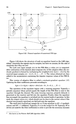
Figure 3.22 Channel equalizer of transversal FIR type

Figure 3.22 shows the structure of such an equalizer based on the LMS algo-
2
rithm . Generally, the signals may be complex, but here we assume, for the sake of
simplicity, that they are real.
For each new input sample x(n) to the FIR filter, a value y(n) is computed.
After subtraction of the desired, ideal response d(ri) of the adaptive filter, the sto-
chastic gradient is formed by multiplying the weighted error o^y(n) - d(n)] by the
received input samples x(n - k), k = 0, 1, ..., N - I. The values obtained are then
added to the accumulators containing the impulse response values of the FIR fil-
ter.
This version of adaptive filter is called a stochastic-gradient equalizer [17].
Updating the filter coefficients proceeds according to

The operation of the equalizer begins with a training sequence. Typically a
periodic sequence whose period equals the length of the FIR filter is sent to the
equalizer through the channel. The same training sequence, properly delayed, is
generated at the receiver and fed into the equalizer. Finally, when the equalizer
has converged, the equalizer is switched into the normal mode of operation. In this
mode the output values y(n\ which should now be close to the correct values if the
channel was properly equalized, are fed back into the equalizer.
The work load involved per sample for an N-tap equalizer is 2N + 3 multipli-
cations and 2N + 1 additions. Typically, N is in the range 8 to 32. Typically, 20 to
24 bits are used for the filter coefficients in order to provide the necessary dynamic

2
' Also known as the Widrow-Hoff LMS algorithm (1960).