Page 94 - DSP Integrated Circuits

3.12 Signal-Flow Graphs 79

The transfer function for an LSI system is a rational function in z and can
therefore be described by a constant gain factor and the roots of the numerator
and denominator. For example, the transfer function of the digital lowpass filter
designed in Example 3.4 is

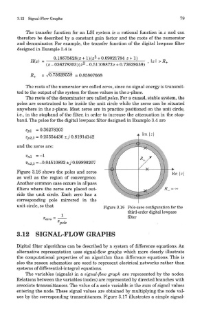
The roots of the numerator are called zeros, since no signal energy is transmit-
ted to the output of the system for those values in the z-plane.
The roots of the denominator are called poles. For a causal, stable system, the
poles are constrained to be inside the unit circle while the zeros can be situated
anywhere in the 2-plane. Most zeros are in practice positioned on the unit circle,
i.e., in the stopband of the filter, in order to increase the attenuation in the stop-
band. The poles for the digital lowpass filter designed in Example 3.4 are

Figure 3.16 shows the poles and zeros
as well as the region of convergence.
Another common case occurs in allpass
filters where the zeros are placed out-
side the unit circle. Each zero has a
corresponding pole mirrored in the
unit circle, so that Figure 3.16 Pole-zero configuration for the
third-order digital lowpass
filter

3.12 SIGNAL-FLOW GRAPHS

Digital filter algorithms can be described by a system of difference equations. An
alternative representation uses signal-flow graphs which more clearly illustrate
the computational properties of an algorithm than difference equations. This is
also the reason schematics are used to represent electrical networks rather than
systems of differential-integral equations.
The variables (signals) in a signal-flow graph are represented by the nodes.
Relations between the variables (nodes) are represented by directed branches with
associate transmittances. The value of a node variable is the sum of signal values
entering the node. These signal values are obtained by multiplying the node val-
ues by the corresponding transmittances. Figure 3.17 illustrates a simple signal-