Page 102 - DSP Integrated Circuits

3.16 FFT—The Fast Fourier Transform Algorithm 87

and the inverse discrete Fourier transform (IDFT) is

where W = e~J 2n/N . Generally, both x(n) and X(k) are complex sequences of length
N. Also note that the discrete Fourier transform is a proper transform. It is not an
approximation of the discrete-time Fourier transform of a sequence that was dis-
cussed earlier. However, the two transforms are closely related.
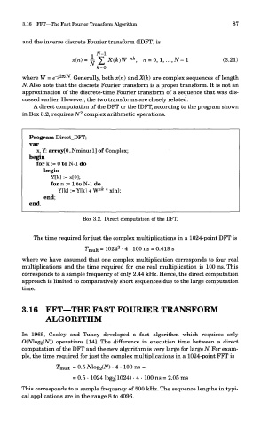
A direct computation of the DFT or the IDFT, according to the program shown
2
in Box 3.2, requires N complex arithmetic operations.

Program Direct_DFT;
var
x, Y: array[O..Nmimisl] of Complex;
begin
for k := 0 to N-l do
begin
Y[k] := x[0];
for n := 1 to N-l do
nk
Y[k] := Y[k] + W * x[n];
end;
end.

Box 3.2. Direct computation of the DFT.

The time required for just the complex multiplications in a 1024-point DFT is
2
^mult = 1024 • 4 • 100 ns = 0.419 s
where we have assumed that one complex multiplication corresponds to four real
multiplications and the time required for one real multiplication is 100 ns. This
corresponds to a sample frequency of only 2.44 kHz. Hence, the direct computation
approach is limited to comparatively short sequences due to the large computation
time.

3.16 FFT—THE FAST FOURIER TRANSFORM
ALGORITHM

In 1965, Cooley and Tukey developed a fast algorithm which requires only
O(Mog2(AO) operations [14]. The difference in execution time between a direct
computation of the DFT and the new algorithm is very large for large N. For exam-
ple, the time required for just the complex multiplications in a 1024-point FFT is

TVnult = 0.5 Mog 2(AO • 4 • 100 ns =
= 0.5 • 1024 Iog 2(1024) • 4 • 100 ns = 2.05 ms
This corresponds to a sample frequency of 500 kHz. The sequence lengths in typi-
cal applications are in the range 8 to 4096.