Page 244 - DSP Integrated Circuits

6.3 Precedence Graphs 229

therefore important that the algorithms at the different hierarchical levels are
carefully designed in order to achieve a high overall system performance.

6.3 PRECEDENCE GRAPHS

A signal-flow graph representation of a DSP algorithm is not directly suitable for
analysis of its computational properties. We will therefore map the signal-flow
graph to other graphs that can better serve to analyze computational properties
such as parallelism and minimum execution time.
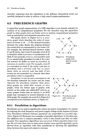
The graph shown in Figure 6.4 is a prece-
dence graph which describes the order of occur-
rence of events: A, B, ..., F. The directed branches
between the nodes denote the ordering between
the events that are represented by the nodes [12].
For example, the directed branch between nodes
E and B shows that event E precedes event B. E
is therefore called a precedent or predecessor to B.
Node E also precedes event A, and therefore node Figure 6.4 Precedence
E is a second-order precedent to node A. In a sim- graph with
ilar manner, we define an event as succedent, or activity on the
successor, to another event. For example, event B nodes
is a succedent to event E. An initial node has no
precedents and a terminal node has no succe-
dents, while an internal node has both. If two
events are not connected via a branch, then their
precedence order is unspecified.
Sometimes, it may be more convenient to let
the branches represent the events and the nodes
represent the precedence relations. Such prece-
dence graphs are called AOA (activity on arcs}
graphs, while the former type of graphs, with
activity on the nodes, are called AON (activity on
nodes) graphs. Notice that an activity in an AON
graph may correspond to several branches in an Figure 6.5 Precedence graph
AOA graph. For example, the event E in Figure 6.4 with activity on
corresponds to two branches shown in Figure 6.5. arcs

6.3.1 Parallelism in Algorithms
Parallelism can be used to significantly reduce the power consumption of a system
by reducing the clock frequency and power supply voltage at the expense of silicon
area. Precedence relations between operations are unspecified in a parallel algo-
rithm. Figure 6.6 illustrates two examples of parallel algorithms. In the first case,
the additions have a common precedent, while in the second case they are inde-
pendent. Two operations (algorithms) are concurrent if their execution times over-
lap. We will later show that in some cases, another more parallel algorithm can be
derived from an algorithm with little parallelism by allowing the algorithmic
delay between the input and output to increase.