Page 245 - DSP Integrated Circuits

230 Chapter 6 DSP Algorithms

Additional computational parallelism may
also appear at both the lower and higher system
levels illustrated in Figure 6.1 [8]. At the lower
level, several bits of an arithmetic operation
may be computed in parallel. At a higher level
(for example, in a DCT-based image processing
system), several rows in a 2-D DCT may be com-
puted concurrently. At a still higher level, sev-
eral DCTs may be computed concurrently.
Hence, large amounts of parallelism and concur-
rency may be present in a particular DSP sys- Figure 6.6 Parallel algorithms
tem, but are often difficult to detect and
therefore difficult to exploit.
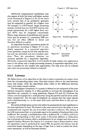
An algorithm having a precedence graph for
its operations according to Figure 6.7 is com-
pletely sequential. In a sequential algorithm
every operation, except for the first and the last,
has only one precedent and one succedent oper- Figure 6.7 Sequential
ation. Thus, the precedence relations are algorithm
uniquely specified for a sequential algorithm.
Obviously, a sequential algorithm is not suitable for high sample rate applications
since it can utilize only a single processing element. A sequential algorithm, how-
ever, is useable for low sample rate applications. The chip area can be reduced
since only one processing element is required.

6.3.2 Latency

We define latency of an algorithm as the time it takes to generate an output value
from the corresponding input value. Note that latency refers to the time between
input and output, while the algorithmic delay refers to the difference between
input and output sample indices.
The throughput (samples/s) of a system is defined as the reciprocal of the time
between successive outputs. It is often possible to increase the throughput of an
algorithm—for example, by using pipelining. Figures 6.8 and 6.9 illustrate the
latency and throughput for a multiplication using bit-parallel and bit-serial arith-
metic, respectively. For the sake of simplicity we assume that the input signals
arrive simultaneously, i.e., in the same clock cycle, and that there is only one out-
put signal.
Bit-serial multiplication can be done either by processing the least significant or
the most significant bit first. The former is the most common since the latter is more
complicated and requires the use of so-called redundant arithmetic. The latency, if
the LSB is processed first, is in principle equal to the number of fractional bits in the
coefficient. For example, a multiplication with a coefficient W c = (1.0011)2 will have
a latency corresponding to four clock cycles. A bit-serial addition or subtraction
has in principle zero latency while a multiplication by an integer may have zero or
negative latency. However, the latency in a recursive loop is always positive, since
the operations must be performed by causal PEs. In practice the latency may be
somewhat longer, depending on the type of logic that is used to realize the arith-
metic operations, as will be discussed shortly.