Page 332 - DSP Integrated Circuits

7.6 Scheduling Algorithms 317

EXAMPLE 7.5
Calculate the forces in the preceding example.
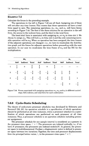
The operations to the left in Figure 7.42 are all fixed. Assigning one of these
will not alter any time frames. This means that these operations all have a total
force equal to zero. The remaining operations, mi, m%, and ai, will have forces
according to Figure 7.44. The first of the three columns for an operation is the self
force, the second is the indirect force, and the third is the total force.
The least total force is associated with assigning mi or 7712 to time slot 3. We
choose to assign mi. This will lock ai to time slot 4 and the only remaining move-
able operation will be m^. When an operation has been assigned, the time frames
of the adjacent operations are changed—i.e., we have to recalculate the distribu-
tion graph and the forces for adjacent operations before proceeding with the next
operation. In our case we recalculate the time frame of m^ and the DG for the
multiplication.

mi ni2 ai
Self Indirect Total Self Indirect Total Self Indirect Total

I o ± ± 0 I I - -
~~1 1 U
3 3 3 ° 3
o _ ? _ 1 _ 5 _ 2 _ 1 _ 5 1 8 „
3 6 6 3 6 6 3 3

<? _ 2 _ 2 _ 4 _ 2 _ 2 _ 4 4 2 -
3 3 3 3 3 3 3 3

« - - - - - - - I o - I

Figure 7.44 Forces associated with assigning operations mi, m%, and a\ to different control
steps. Self, indirect, and total force for each combination

7.6.6 Cyclo-Static Scheduling
The theory of cyclo-static processor schedules was developed by Schwartz and
Barnwell [22, 23]. An operation schedule is a specification of which operations
should be performed at all time instances, while a processor schedule is a speci-
fication of which operations are performed on each processor at all time
instances. Thus, a processor schedule is an operation schedule including proces-
sor assignment.
The processor schedule for one sample interval is considered as a pattern in
the processor-time space, P x T. The processors are indexed cyclically, i.e., if we
have N processors, the processors are indexed modulo(AT). In general, the proces-
sor space is multidimensional. Further, a displacement vector is defined in proces-
sor space between two iterations. Together, the time and processor displacements
form the principal lattice vector, L, in the processor-time space IP x T.