
Page 335 - DSP Integrated Circuits
P. 335
320 Chapter 7 DSP System Design
7.6.7 Maximum Spanning Tree Method
The maximum spanning tree method, which was developed by Renfors and Neuvo
[20], can be used to achieve rate optimal schedules. The method is based on graph-
theoretical concepts. The starting point is the fully specified SFG. The SFG corre-
sponds to a computation graph N, which is formed by inserting the operation
delays into the SFG. Further, a new graph N' is formed from N by replacing the
delay elements by negative delay elements (-T). In this graph we find the maxi-
mum distance spanning tree—i.e., a spanning tree where the distance from the
input to each node is maximal. Next, shimming delays are inserted in the link
branches (i.e., the remaining branches) so that the total delay in the loops becomes
zero. Finally, remove the negative delays. The remaining delays, apart from the
operation delays, are the shimming delays. These concepts are described by an
example.
EXAMPLE 7.7
Consider the second-order section as in Example 7.6 and derive a rate optimal
schedule using the maximum spanning tree method.
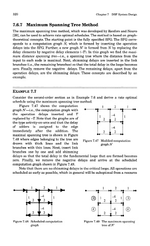
Figure 7.47 shows the computation
graph N'—i.e., the computation graph with
the operation delays inserted and T
replaced by — T. Note that the graphs are of
the type activity-on-arcs and that the delay
of adders is assigned to the edge
immediately after the addition. The
maximal spanning tree is shown in Figure
7.48 where edges belonging to the tree are
Figure 7.47 Modified computation
drawn with thick lines and the link graph N'
branches with thin lines. Next, insert link
branches one by one and add shimming
delays so that the total delay in the fundamental loops that are formed becomes
zero. Finally, we remove the negative delays and arrive at the scheduled
computation graph shown in Figure 7.49.
Note that there are no shimming delays in the critical loops. All operations are
scheduled as early as possible, which in general will be suboptimal from a resource
Figure 7.48 Scheduled computation Figure 7.49 The maximum spanning
graph tree of AT