Page 337 - DSP Integrated Circuits

322 Chapter 7 DSP System Design

Program Simulated_Annealing;

begin
Initialize;
M:=0;
repeat
repeat
Perturb(state(i) -> state(k), ACost(i, k));
if ACost(i, k) < 0 then accept
else
if exp(-ACost(i, k)/T]vi) > Random(0,1) then accept;
if accept then Update(state(k));
until Equilibrium; {Sufficiently close }
TM+I := #TM);
M:=M+1;
until Stop_Criterion = True; {System is frozen }
end.

Box 7.6 Simulated annealing algorithm

The algorithm starts from a valid solution (state) and randomly generates new
states, stated), for the problem and calculates the associated cost function, Cost(i).
Simulation of the annealing process starts at a high fictitious temperature, TM- A
new state, k, is randomly chosen and the difference in cost is calculated, ACostd, k).
If ACostd, k) < 0, i.e., the cost is lower, then this new state is accepted. This forces
the system toward a state corresponding to a local or possibly a global minimum.
However, most large optimization problems have many local minima and the opti-
mization algorithm is therefore often trapped in a local minimum.
To get out of a local minimum, an increase of the cost function is accepted with
a certain probability—i.e., if

then the new state is accepted. The simula-
tion starts with a high temperature, TM- This
makes the left-hand side of Equation (7.7)
close to 1. Hence, a new state with a larger
cost has a high probability of being accepted.
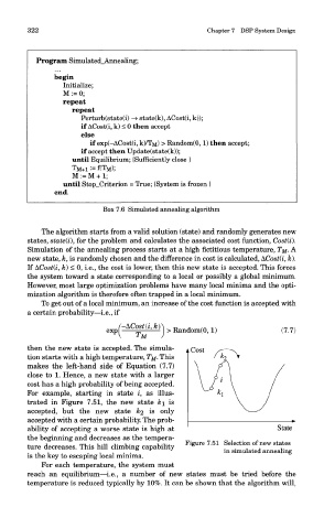
For example, starting in state i, as illus-
trated in Figure 7.51, the new state k\ is
accepted, but the new state &2 is on ty
accepted with a certain probability. The prob-
ability of accepting a worse state is high at
the beginning and decreases as the tempera-
Figure 7.51 Selection of new states
ture decreases. This hill climbing capability in simulated annealing
is the key to escaping local minima.
ror eacn temperature, tne system must
reach an equilibrium—i.e., a number of new states must be tried before the
temperature is reduced typically by 10%. It can be shown that the algorithm will,