Page 164 - Decision Making Applications in Modern Power Systems

128 Decision Making Applications in Modern Power Systems

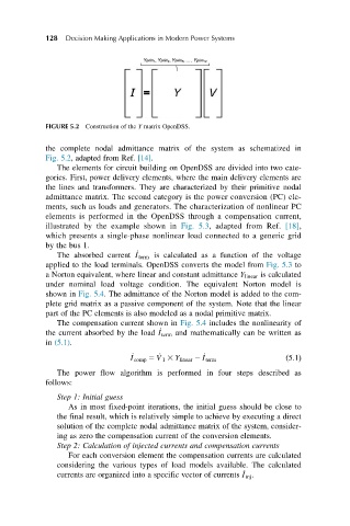
FIGURE 5.2 Construction of the Y matrix OpenDSS.

the complete nodal admittance matrix of the system as schematized in
Fig. 5.2, adapted from Ref. [14].
The elements for circuit building on OpenDSS are divided into two cate-
gories. First, power delivery elements, where the main delivery elements are
the lines and transformers. They are characterized by their primitive nodal
admittance matrix. The second category is the power conversion (PC) ele-
ments, such as loads and generators. The characterization of nonlinear PC
elements is performed in the OpenDSS through a compensation current,
illustrated by the example shown in Fig. 5.3, adapted from Ref. [18],
which presents a single-phase nonlinear load connected to a generic grid
by the bus 1.
_
The absorbed current I term is calculated as a function of the voltage
applied to the load terminals. OpenDSS converts the model from Fig. 5.3 to
a Norton equivalent, where linear and constant admittance Y linear is calculated
under nominal load voltage condition. The equivalent Norton model is
shown in Fig. 5.4. The admittance of the Norton model is added to the com-
plete grid matrix as a passive component of the system. Note that the linear
part of the PC elements is also modeled as a nodal primitive matrix.
The compensation current shown in Fig. 5.4 includes the nonlinearity of
_
the current absorbed by the load I term and mathematically can be written as
in (5.1).
_ _ _
I comp 5 V 1 3 Y linear 2 I term ð5:1Þ
The power flow algorithm is performed in four steps described as
follows:

Step 1: Initial guess
As in most fixed-point iterations, the initial guess should be close to
the final result, which is relatively simple to achieve by executing a direct
solution of the complete nodal admittance matrix of the system, consider-
ing as zero the compensation current of the conversion elements.
Step 2: Calculation of injected currents and compensation currents
For each conversion element the compensation currents are calculated
considering the various types of load models available. The calculated
_
currents are organized into a specific vector of currents I inj .