Page 290 - Decision Making Applications in Modern Power Systems

250 Decision Making Applications in Modern Power Systems

V
Predictor Corrector

P P
max
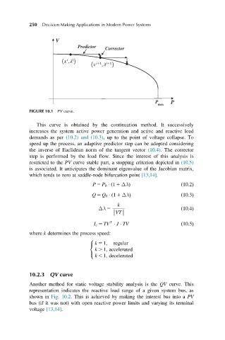
FIGURE 10.1 PV curve.

This curve is obtained by the continuation method. It successively
increases the system active power generation and active and reactive load
demands as per (10.2) and (10.3), up to the point of voltage collapse. To
speed up the process, an adaptive predictor step can be adopted considering
the inverse of Euclidean norm of the tangent vector (10.4). The corrector
step is performed by the load flow. Since the interest of this analysis is
restricted to the PV curve stable part, a stopping criterion depicted in (10.5)
is associated. It anticipates the dominant eigenvalue of the Jacobian matrix,
which tends to zero at saddle-node bifurcation point [13,14].

P 5 P 0 ð1 1 ΔλÞ ð10:2Þ
Q 5 Q 0 ð1 1 ΔλÞ ð10:3Þ
k
Δλ 5 ð10:4Þ
:VT:

T
I c 5 TV J TV ð10:5Þ
where k determines the process speed:
8
k 5 1; regular
<
k . 1; accelerated
k , 1; decelerated
:

10.2.3 QV curve
Another method for static voltage stability analysis is the QV curve. This
representation indicates the reactive load range of a given system bus, as
shown in Fig. 10.2. This is achieved by making the interest bus into a PV
bus (if it was not) with open reactive power limits and varying its terminal
voltage [13,14].