Page 286 - Design and Operation of Heat Exchangers and their Networks

272 Design and operation of heat exchangers and their networks

procedures. Such examples are summarized in the succeeding text with their
up-to-date global minimum of TAC and the corresponding structures.
We will label such examples with the number of hot streams and cold
streams. Each example is revised according to the given optimal network
configuration and original problem data, calculated with the exact equation
of logarithmic mean temperature difference, and optimized to its local min-
imum of TAC using a local optimizing strategy (Luo et al., 2009).

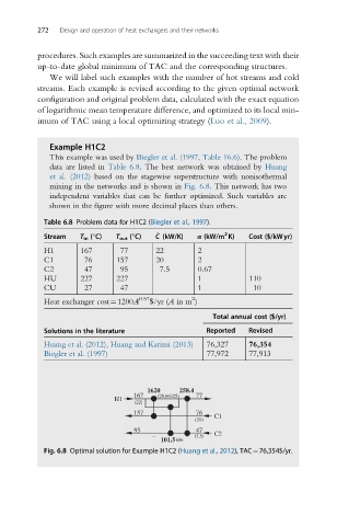
Example H1C2
This example was used by Biegler et al. (1997, Table 16.6). The problem
data are listed in Table 6.8. The best network was obtained by Huang
et al. (2012) based on the stagewise superstructure with nonisothermal
mixing in the networks and is shown in Fig. 6.8. This network has two
independent variables that can be further optimized. Such variables are
shown in the figure with more decimal places than others.

Table 6.8 Problem data for H1C2 (Biegler et al., 1997).
2
_
Stream T in (°C) T out (°C) C (kW/K) α (kW/m K) Cost ($/kWyr)
H1 167 77 22 2
C1 76 157 20 2
C2 47 95 7.5 0.67
HU 227 227 1 110
CU 27 47 1 10
2
Heat exchanger cost¼1200A 0.57 $/yr (A in m )
Total annual cost ($/yr)
Solutions in the literature Reported Revised

Huang et al. (2012), Huang and Karimi (2013) 76,327 76,354
Biegler et al. (1997) 77,972 77,913

1620 258.4
167 (20.66325) 77
H1
(22)
157 76
C1
(20)
95 47
(7.5) C2
101.5686
Fig. 6.8 Optimal solution for Example H1C2 (Huang et al., 2012), TAC¼76,354$/yr.