Page 287 - Design and Operation of Heat Exchangers and their Networks

Optimal design of heat exchanger networks 273

Example H2C1
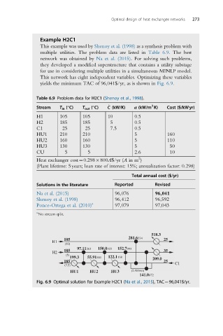
This example was used by Shenoy et al. (1998) as a synthesis problem with
multiple utilities. The problem data are listed in Table 6.9. The best
network was obtained by Na et al. (2015). For solving such problems,
they developed a modified superstructure that contains a utility substage
for use in considering multiple utilities in a simultaneous MINLP model.
This network has eight independent variables. Optimizing these variables
yields the minimum TAC of 96,041$/yr, as is shown in Fig. 6.9.

Table 6.9 Problem data for H2C1 (Shenoy et al., 1998).
2
_
Stream T in (°C) T out (°C) C (kW/K) α (kW/m K) Cost ($/kWyr)
H1 105 105 10 0.5
H2 185 185 5 0.5
C1 25 25 7.5 0.5
HU1 210 210 5 160
HU2 160 160 5 110
HU3 130 130 5 50
CU 5 5 2.6 10
2
Heat exchanger cost¼0.298 800A$/yr (A in m )
(Plant lifetime: 5years; loan rate of interest: 15%; annualization factor: 0.298)
Total annual cost ($/yr)
Solutions in the literature Reported Revised
Na et al. (2015) 96,076 96,041
Shenoy et al. (1998) 96,412 96,592
Ponce-Ortega et al. (2010) a 97,079 97,043
a
No stream split.

518.3
281.6 534
105 25
H1
(10)
97.11 261 150.0 322 152.7 995
185 35
H2
(5)
199.3 55.91 801 122.1 138 209.0
185 25
(7.5) C1
HU1 HU2 HU3 (2.503083)
141.0 872
Fig. 6.9 Optimal solution for Example H2C1 (Na et al., 2015), TAC¼96,041$/yr.