Page 292 - Design and Operation of Heat Exchangers and their Networks

278 Design and operation of heat exchangers and their networks

Example H2C2_300
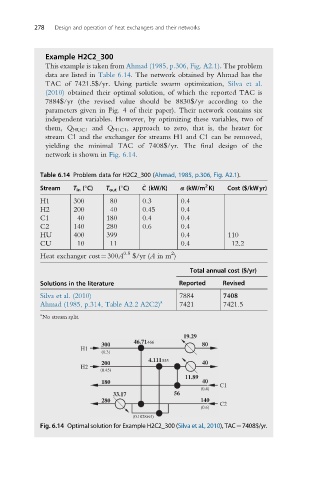
This example is taken from Ahmad (1985, p.306, Fig. A2.1). The problem
data are listed in Table 6.14. The network obtained by Ahmad has the
TAC of 7421.5$/yr. Using particle swarm optimization, Silva et al.
(2010) obtained their optimal solution, of which the reported TAC is
7884$/yr (therevised valueshould be8830$/yr according to the
parameters given in Fig. 4 of their paper). Their network contains six
independent variables. However, by optimizing these variables, two of
them, Q HUC1 and Q H1C1 , approach to zero, that is, the heater for
stream C1 and the exchanger for streams H1 and C1 can be removed,
yielding the minimal TAC of 7408$/yr. The final design of the
network is shown in Fig. 6.14.

Table 6.14 Problem data for H2C2_300 (Ahmad, 1985, p.306, Fig. A2.1).
2
_
Stream T in (°C) T out (°C) C (kW/K) α (kW/m K) Cost ($/kWyr)
H1 300 80 0.3 0.4
H2 200 40 0.45 0.4
C1 40 180 0.4 0.4
C2 140 280 0.6 0.4
HU 400 399 0.4 110
CU 10 11 0.4 12.2
2
Heat exchanger cost¼300A 0.5 $/yr (A in m )
Total annual cost ($/yr)
Solutions in the literature Reported Revised

Silva et al. (2010) 7884 7408
Ahmad (1985, p.314, Table A2.2 A2C2) a 7421 7421.5
a
No stream split.
19.29
46.71 466
300 80
H1
(0.3)
4.111 555
200 40
H2
(0.45)
11.89
180 40
C1
(0.4)
33.17 56
280 140
C2
(0.6)
(0.1028495)
Fig. 6.14 Optimal solution for Example H2C2_300 (Silva et al., 2010), TAC¼7408$/yr.