Page 296 - Design and Operation of Heat Exchangers and their Networks

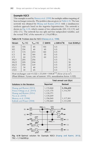
282 Design and operation of heat exchangers and their networks

Example H2C3
This example is used by Shenoy et al. (1998) for multiple utilities targeting of
heat exchanger networks. The problem data are given in Table 6.18.The best
network was obtained by Huang and Karimi (2013) with a simultaneous
synthesis approach based on the stagewise hyperstructure. The network is
shown in Fig. 6.18, which consists of two subnetworks {H1, C2, C3} and
{H2, C1}. The network has one split and four independent variables, and
the revised TAC of the network is 1,116,629$/yr.
Table 6.18 Problem data for H2C3 (Shenoy et al., 1998).
2
_
Stream T in (°C) T out (°C) C (kW/K) α (kW/m K) Cost ($/kWyr)
H1 155 85 150 0.5
H2 230 40 85 0.5
C1 115 210 140 0.5
C2 50 180 55 0.5
C3 60 175 60 0.5
HU1 255 254 0.5 70
HU2 205 204 0.5 50
HU3 150 149 0.5 20
CU1 30 40 0.5 10
CU2 40 65 0.5 5
2
Heat exchanger cost¼0.322 (13,000+1000A 0.83 ) $/yr (A in m )
(Plant lifetime: 5years; rate of interest: 10%; annualization factor: 0.322)
Total annual cost ($/yr)
Solutions in the literature Reported Revised

Huang and Karimi (2013) 1,115,868 1,116,630
Ponce-Ortega et al. (2010) 1,121,175 1,116,787
Huang and Karimi (2014) 1,120,271
Na et al. (2015) 1,120,609
Shenoy et al. (1998) 1,158,500 1,117,381
Isafiade and Fraser (2008) 1,150,460 1,121,698

5066. 436 CU1
155 (72.26217) 512 85
H1
(150)
7047
230 40
H2 (85)
4197 CU1
210 115
C1
HU1 9102. 914 (140)
2084
180 50
C2
HU2 (55)
175 60
C3
HU2 4921. (60)
1979 479
Fig. 6.18 Optimal solution for Example H2C3 (Huang and Karimi, 2013),
TAC¼1,116,630$/yr.