Page 299 - Design and Operation of Heat Exchangers and their Networks

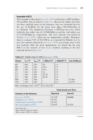
Optimal design of heat exchanger networks 285

Example H3C3
This example is taken from Lee et al. (1970) and known as 6SP1 problem.
Theproblem data arelistedin Table 6.21. Because the utility costs have
not been explicitly given in the literature, they are calculated here by
the use of RefProp for the latent heat (Δh fg ¼768.33Btu/lbm at
p s ¼450psia). The equipment downtime is 380hours per year, which
yields the hot utility cost of 10.906$/kBtu/yr and the cold utility cost
of 5.2375$/kBtu/yr, respectively. The best network was found by
Nishida et al. (1977), which has no independent variable. Therefore,
there is a unique TAC of 35,010$/yr, as is reported by Nishida et al. In
fact, the network obtained by Lee et al. (1970) was already close to this
best network. After the local optimization, we found that the unit
H2C2 in the network of Lee et al. vanished, resulting to the best
network shown in Fig. 6.21.

Table 6.21 Problem data for H3C3 (Lee et al., 1970).
2
_
Stream T in (°F) T out (°F) C (kBtu/h°F) α (kBtu/ft °F) Cost ($/kBtuyr)
H1 440 150 28 0.3
H2 520 300 23.8 0.3
H3 390 150 33.6 0.3
C1 100 430 16 0.3
C2 180 350 32.76 0.3
C3 200 400 26.35 0.3
HU 456 456 0.6 10.906
CU 100 180 0.3 5.2375
0.6 2
Heat exchanger cost¼35A $/yr (A in ft )
Total annual cost ($/yr)

Solutions in the literature Reported Revised
Lee et al. (1970) a 35,108 b 35,010
Nishida et al. (1977) a 35,010
Chakraborty and Ghosh (1999) a 35,016
Pho and Lapidus (1973) a 35,659 c 35,526
a
No stream split.
b
After revision, H2C2 is deleted.
c
After revision, H2CU is deleted.
Continued