Page 291 - Design and Operation of Heat Exchangers and their Networks

Optimal design of heat exchanger networks 277

Example H2C2_270
This example was originally introduced by Gundersen (2002). The problem
data were given by Escobar and Trierweiler (2013) and are listed in
Table 6.13. They used the General Algebraic Modeling System (GAMS)
to solve this problem. However, their solutions did not approach to the
local minimal TAC of the corresponding networks. After the optimization
of the independent variables, in their network shown in Fig. A2(b) of
their paper, the bypass of H1 after the exchanger H1C2 is eliminated, and
the TAC of the network approaches to 351,411$/yr. Later, the better
solution was found by Stegner et al. (2014) by the use of an enhanced
vertical heat exchange algorithm, in which a new form of graphic
depiction of the problem’s data in a temperature-enthalpy diagram was
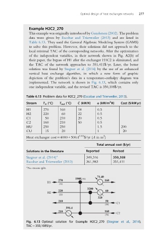
implemented. The network is shown in Fig. 6.13, which contains only
one independent variable, and the revised TAC is 350,108$/yr.

Table 6.13 Problem data for H2C2_270 (Escobar and Trierweiler, 2013).
_
2
Stream T in (°C) T out (°C) C (kW/K) α (kW/m K) Cost ($/kWyr)
H1 270 160 18 0.5
H2 220 60 22 0.5
C1 50 210 20 0.5
C2 160 210 50 0.5
HU 250 250 1.5 200
CU 15 20 1 20
2
Heat exchanger cost¼4000+500A 0.83 $/yr (A in m )
Total annual cost ($/yr)
Solutions in the literature Reported Revised
Stegner et al. (2014) a 349,316 350,108
Escobar and Trierweiler (2013) 361,983 351,411
a
No stream split.
71.40
1908. 598
270 160
H1
(18)
3200
220 60
H2
(22)
320
210 50
C1
(20)
591.4
210 160
C2
(50)
Fig. 6.13 Optimal solution for Example H2C2_270 (Stegner et al., 2014),
TAC¼350,108$/yr.