Page 290 - Design and Operation of Heat Exchangers and their Networks

276 Design and operation of heat exchangers and their networks

Example H2C2_260
This example was originally introduced by Ahmad (1985, p. 315,
Fig. A2.15), in which the heat transfer coefficients for all matches were
2
1.5kW/m K. Nielsen et al. (1996) used the data for the network design
considering the minimum number of 1–2 shells in an exchanger based
on a specified effectiveness parameter X p ¼0.9. The heat transfer
2
coefficients for all matches were 0.4kW/m K. Khorasany and
Fesanghary (2009) took these data for the network design with common
counterflow heat exchangers. According to the problem data given in
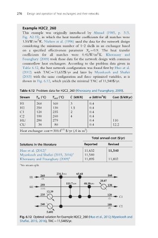
Table 6.12, the best network configuration was found first by Huo et al.
(2012) with TAC¼11,632$/yr and later by Myankooh and Shafiei
(2015) with the same configuration and three optimized variables, as is
shown in Fig. 6.12, which yields the minimal TAC of 11,540$/yr.

Table 6.12 Problem data for H2C2_260 (Khorasany and Fesanghary, 2009).
2
_
Stream T in (°C) T out (°C) C (kW/K) α (kW/m K) Cost ($/kWyr)
H1 260 160 3 0.4
H2 250 130 1.5 0.4
C1 120 235 2 0.4
C2 180 240 4 0.4
HU 280 279 0.4 110
CU 30 80 0.4 12.2
0.5 2
Heat exchanger cost¼300A $/yr (A in m )
Total annual cost ($/yr)
Solutions in the literature Reported Revised

Huo et al. (2012) a 11,632 11,540
Myankooh and Shafiei (2015, 2016) a 11,540
Khorasany and Fesanghary (2009) a 11,895 11,802
a
No stream split.
234.3 191 65.68
260 160
H1
(3)
28.07
111.7 409 40.18 850
250 130
H2
(1.5)
12.39
235 120
C1
(2)
240 180 C2
(4)
5.681
Fig. 6.12 Optimal solution for Example H2C2_260 (Huo et al., 2012; Myankooh and
Shafiei, 2015, 2016), TAC¼11,540$/yr.