Page 87 - Design and Operation of Heat Exchangers and their Networks

Steady-state characteristics of heat exchangers 75

h i
_
_
ð
C h =C c 1 e kA= _ C h + kA= _ C cÞ
00
t t 0
c c
¼ (3.25)
0
t t 0 _ _
h c 1+ C h =C c
The heat load can be calculated either from the hot fluid or from the
cold fluid:
h i
_
ð
C h 1 e kA= _ C h + kA= _ C cÞ

_
_
0
0
00
0
Q ¼ C h t t 00 ¼ C c t t ¼ t t 0
h h c c _ _ h c
1+ C h =C c
(3.26)
Eqs. (3.24)–(3.26) can explicitly offer us the relations
00
t t 00
_
_
ð
0
00
h c 0 ¼ e kA= _ C h + kA= _ C cÞ andkA=C h + kA=C c ¼ kA t t 00 + t t 0 =Q
0
t t h h c c
h c
from which we can express the heat load as

0
0
t t t t 00
00
Q ¼ kA h c h c (3.27)
00
0
ln t t = t t 00 c
0
h
h
c
The subroutines for the calculation of inverse matrix, eigenvalues, and
eigenvectors are available in many source code libraries. These functions
are also included in MatLab. Therefore, the previous calculation is easy to
be carried out.
3.1.2 Counterflow heat exchangers
The same methodology can be applied to the counterflow heat exchangers.
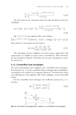
As is shown in Fig. 3.2, in the counterflow heat exchangers, the two fluid flows
are parallel to one another but in opposite directions. The fluid inlets of hot
and cold fluids are at the opposite ends of the exchanger, as well as the fluid
outlets.
For the counterflow heat exchanger, the coefficient matrix in Eq. (3.7)
becomes
" #
_ _
kA=C h kA=C h
A ¼ _ _ (3.28)
kA=C c kA=C c
Fig. 3.2 Heat transfer and temperature variation in a counterflow heat exchanger.