Page 460 - Design for Six Sigma a Roadmap for Product Development

Fundamentals of Experimental Design 419

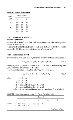
TABLE 12.1 Data of Example 12.2

Glass Phosphor type
type 1 2 3

1 280 300 290
290 310 285
285 295 290
2 230 260 220
235 240 225
240 235 230

12.2.1 The layout of two-factor
factorial experiments
In general, a two-factor factorial experiment has the arrangement
shown in Table 12.2.
Each “cell” of Table 12.2 corresponds to a distinct factor level combi-
nation. In DOE terminology, it is called a “treatment.”

12.2.2 Mathematical model
If we denote A as x 1 and B as x 2 , then one possible mathematical model is
y f 1 (x 1 ) f 2 (x 2 ) f 12 (x 1 , x 2 ) ε (12.2)

Here f 1 (x 1 ) and f 2 (x 2 ) are the main effects of A and B, respectively, and
f 12 (x 1 , x 2 ) is the interaction of A and B.
In many statistics books, the following model is used

(12.3)
y ijk A i B j (AB) ij ε ijk
where i 1,2,…,a
j 1,2,…,b
k 1,2,…,n
A i main effect of A at ith level
B j main effect of B at jth level
(AB) ij interaction effect of A at ith level and B at jth level

TABLE 12.2 General Arrangement for a Two-Factor Factorial Design
Factor B
1 2 … b
Factor A 1 Y 111 , Y 112 , ..., Y 11n Y 121 , Y 122 , ..., Y 12n ...
2 Y 211 , Y 212 , ..., Y 21n ...

a Y ab1, Y ab2, ..., Y abn