Page 464 - Design for Six Sigma a Roadmap for Product Development

Fundamentals of Experimental Design 423

It can be shown that
a b n a b

(y ijk y...) bn
(y i .. y...) an
(y. j . y...) 2
2
2

i 1 j 1 k 1 i 1 j 1
a b

n

(y ij . y i .. y. j . y...) 2

i 1 j 1
a b n

(y ijk y ij .) 2 (12.5)

i 1 j 1 k 1
or simply
(12.6)
SS T SS A SS B SS AB SS E
where SS T is the total sum of squares, which is a measure of the total
variation in the whole data set; SS A is the sum of squares due to A,
which is a measure of total variation caused by main effect of A;SS B is
the sum of squares due to B, which is a measure of total variation
caused by main effect of B;SS AB is the sum of squares due to AB, which
is the measure of total variation due to AB interaction; and SS E is the
sum of squares due to error, which is the measure of total variation due
to error.
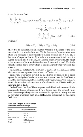
In statistical notation, the number of degree of freedom associated
with each sum of squares is as shown in Table 12.4.
Each sum of squares divided by its degree of freedom is a mean
square. In analysis of variance, mean squares are used in the F test to
see if the corresponding effect is statistically significant. The complete
result of an analysis of variance is often listed in an ANOVA table, as
shown in Table 12.5.
In the F test, the F 0 will be compared with F-critical values with the
appropriate degree of freedom; if F 0 is larger than the critical value,
then the corresponding effect is statistically significant. Many statisti-
cal software programs, such as MINITAB, are convenient for analyzing
DOE data.

TABLE 12.4 Degree of Freedom for
Two-Factor Factorial Design
Effect Degree of freedom
A a 1
B b 1
AB interaction (a 1)(b 1)
Error ab(n 1)
Total abn 1