Page 469 - Design for Six Sigma a Roadmap for Product Development

428 Chapter Twelve

4
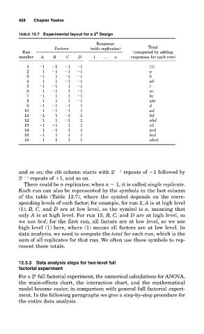
TABLE 12.7 Experimental layout for a 2 Design
Response
Factors (with replicates) Total
Run (computed by adding
number A B C D 1 … n responses for each row)
1 1 1 1 1 (1)
2 1 1 1 1 a
3 1 1 1 1 b
4 1 1 1 1 ab
5 1 1 1 1 c
6 1 1 1 1 ac
7 1 1 1 1 bc
8 1 1 1 1 abc
9 1 1 1 1 d
10 1 1 1 1 ad
11 1 1 1 1 bd
12 1 1 1 1 abd
13 1 1 1 1 cd
14 1 1 1 1 acd
15 1 1 1 1 bcd
16 1 1 1 1 abcd

and so on; the ith column starts with 2 i 1 repeats of 1 followed by
2 i 1 repeats of 1, and so on.
There could be n replicates; when n 1, it is called single replicate.
Each run can also be represented by the symbols in the last column
of the table (Table 12.7), where the symbol depends on the corre-
sponding levels of each factor; for example, for run 2, A is at high level
(1); B, C, and D are at low level, so the symbol is a, meaning that
only A is at high level. For run 15, B, C, and D are at high level, so
we use bcd; for the first run, all factors are at low level, so we use
high level (1) here, where (1) means all factors are at low level. In
data analysis, we need to compute the total for each run, which is the
sum of all replicates for that run. We often use those symbols to rep-
resent those totals.

12.3.3 Data analysis steps for two-level full
factorial experiment
k
For a 2 full factorial experiment, the numerical calculations for ANOVA,
the main-effects chart, the interaction chart, and the mathematical
model become easier, in comparison with general full factorial experi-
ment. In the following paragraphs we give a step-by-step procedure for
the entire data analysis.