Page 472 - Design for Six Sigma a Roadmap for Product Development

Fundamentals of Experimental Design 431

2 k n 2
y...
2
SS T

y ijk (12.10)
i 1 j 1 k 1 N
n
where y ijk is actually each individual response and y... is the sum of all
individual responses.
In Example 12.5

SS T 18.2 18.9 … 39.9 2
2
2
(18.2 18.9 … 39.9) 2
1709.83
16
SS E can be calculated by

SS E SS T SS A SS B SS AB
In Example 12.5
SS E SS T SS A SS B SS AB 1709.83 1107.22 227.25
303.6 71.72

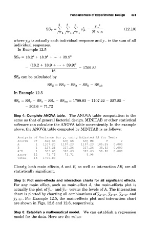
Step 4: Complete ANOVA table. The ANOVA table computation is the
same as that of general factorial design. MINITAB or other statistical
software can calculate the ANOVA table conveniently. In the example
above, the ANOVA table computed by MINITAB is as follows:

Analysis of Variance for y, using Adjusted SS for Tests
Source DF Seq SS Adj SS Adj MS F P
A 1 1107.23 1107.23 1107.23 185.25 0.000
B 1 227.26 227.26 227.26 38.02 0.000
A*B 1 303.63 303.63 303.63 50.80 0.000
Error 12 71.72 71.72 5.98
Total 15 1709.83

Clearly, both main effects, A and B, as well as interaction AB, are all
statistically significant.

Step 5: Plot main-effects and interaction charts for all significant effects.
For any main effect, such as main-effect A, the main-effects plot is
actually the plot of y A and y A versus the levels of A. The interaction

chart is plotted by charting all combinations of y A B , y A B , y A B and

y A B . For Example 12.5, the main-effects plot and interaction chart
are shown in Figs. 12.5 and 12.6, respectively.
Step 6: Establish a mathematical model. We can establish a regression
model for the data. Here are the rules: