Page 470 - Design for Six Sigma a Roadmap for Product Development

Fundamentals of Experimental Design 429

Step 0: Preparation
Establish analysis matrix for the problem. The analysis matrix is a matrix
that has not only all columns for factors but also the columns for all
interactions. The interaction columns are obtained by multiplying the
corresponding columns of factors involved. For example, in a 2 exper-
2
iment, the analysis matrix is as follows, where the AB column is gen-
erated by multiplying the A and B columns:

Run number A B AB
*
1 1 1 ( 1) ( 1) 1
2 1 1 ( 1) * ( 1) 1
3 1 1 ( 1) * ( 1) 1
*
4 1 1 ( 1) ( 1) 1
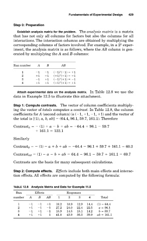
Attach experimental data on the analysis matrix. In Table 12.8 we use the
data in Example 12.5 to illustrate this attachment.

Step 1: Compute contrasts. The vector of column coefficients multiply-
ing the vector of totals computes a contrast. In Table 12.8, the column
coefficients for A (second column) is ( 1, 1, 1, 1) and the vector of
the total is [(1), a, b, ab] (64.4, 96.1, 59.7, 161.1). Therefore

Contrast A (1) a b ab 64.4 96.1 59.7
161.1 133.1

Similarly

Contrast B (1) a b ab 64.4 96.1 59.7 161.1 60.3
Contrast AB (1) a b ab 64.4 96.1 59.7 161.1 69.7

Contrasts are the basis for many subsequent calculations.

Step 2: Compute effects. Effects include both main effects and interac-
tion effects. All effects are computed by the following formula:

TABLE 12.8 Analysis Matrix and Data for Example 11.5
Run Effects Responses
number A B AB 1 2 3 4 Total
1 1 1 1 18.2 18.9 12.9 14.4 (1) 64.4
2 1 1 1 27.2 24.0 22.4 22.5 a 96.1
3 1 1 1 15.9 14.5 15.1 14.2 b 59.7
4 1 1 1 41.0 43.9 36.3 39.9 ab 161.1