Page 554 - Design for Six Sigma a Roadmap for Product Development

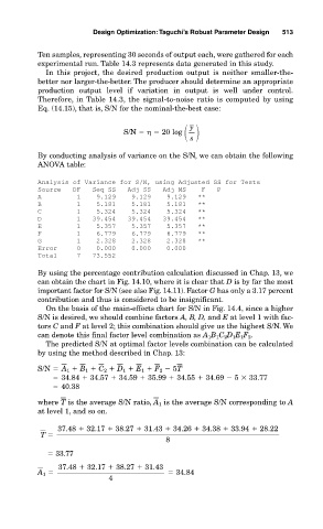
Design Optimization:Taguchi’s Robust Parameter Design 513

Ten samples, representing 30 seconds of output each, were gathered for each
experimental run. Table 14.3 represents data generated in this study.
In this project, the desired production output is neither smaller-the-
better nor larger-the-better. The producer should determine an appropriate
production output level if variation in output is well under control.
Therefore, in Table 14.3, the signal-to-noise ratio is computed by using
Eq. (14.15), that is, S/N for the nominal-the-best case:

y

S/N 20 log
s
By conducting analysis of variance on the S/N, we can obtain the following
ANOVA table:
Analysis of Variance for S/N, using Adjusted SS for Tests
Source DF Seq SS Adj SS Adj MS F P
A 1 9.129 9.129 9.129 **
B 1 5.181 5.181 5.181 **
C 1 5.324 5.324 5.324 **
D 1 39.454 39.454 39.454 **
E 1 5.357 5.357 5.357 **
F 1 6.779 6.779 6.779 **
G 1 2.328 2.328 2.328 **
Error 0 0.000 0.000 0.000
Total 7 73.552
By using the percentage contribution calculation discussed in Chap. 13, we
can obtain the chart in Fig. 14.10, where it is clear that D is by far the most
important factor for S/N (see also Fig. 14.11). Factor G has only a 3.17 percent
contribution and thus is considered to be insignificant.
On the basis of the main-effects chart for S/N in Fig. 14.4, since a higher
S/N is desired, we should combine factors A, B, D, and E at level 1 with fac-
tors C and F at level 2; this combination should give us the highest S/N. We
can denote this final factor level combination as A 1 B 1 C 2 D 1 E 1 F 2 .
The predicted S/N at optimal factor levels combination can be calculated
by using the method described in Chap. 13:
S/N A 1 B 1 C 2 D 1 E 1 F 2 5T
34.84 34.57 34.59 35.99 34.55 34.69 5
33.77
40.38
where T is the average S/N ratio, A 1 is the average S/N corresponding to A
at level 1, and so on.

37.48 32.17 38.27 31.43 34.26 34.38 33.94 28.22
T
8
33.77
37.48 32.17 38.27 31.43
A 1 34.84
4