Page 639 - Design for Six Sigma a Roadmap for Product Development

592 Chapter Sixteen

0.20
"C L
p L 0.678
("f) 2 L 0.295
Because

∂f

("f) R "R 0.948
0.5 0.474 A
∂R

∂f
("f) L "L 0.98.53
0.003 0.295 A
"L
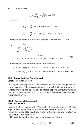
Therefore, reducing R is more cost-effective than reducing L. Then

req
p
i 1 ∂x i 2
n

2

∂f
2
p i
i
0.1667
1.332
0.316
0. 899
0.25 0.6 78
9708.2
0 .0015 2

2
2
2
Therefore, the new tolerance limits for R and L are
R 3C p pp R R 3
1.333
1.332
0.316
0.25 0.42
L 3C p pp L L 3
1.333
1.332
0.678
0.0015 0.0054 H
16.5 Taguchi’s Loss Function and
Safety Tolerance Design
Dr. Taguchi developed a unique approach to tolerance design and tol-
erance analysis. His tolerance design approach includes a cost-based
tolerance design and allocation. The most important consideration in
cost is the quality loss due to requirement deviation from the ideal
requirement level.

16.5.1 Customer tolerance and
producer tolerance
Nominal-the-best requirement. The quality loss can be expressed by the
Taguchi quality loss function that we discussed in detail in Chap. 14.
Figure 16.8 shows the quadratic curve for the quality loss function for
the “nominal-the-best” case.
The quality loss function can be expressed as follows:

A 0
L(y) (y T) 2 (16.29)
2
0