Page 637 - Design for Six Sigma a Roadmap for Product Development

590 Chapter Sixteen

Step 1. Identify the exact transfer function between high-level
requirement y and low-level characteristics; that is, identify the
equation y f(x 1 ,x 2 ,…,x i ,…,x n ). If the equation is not given in closed
form, we can use a computer simulation model, or an empirical model
derived from a DOE study.
...
Step 2. For each low-level characteristic x i , i 1 n, identify its
i , C p , and i . This can be done by analyzing historical process
control data, if x i is made by an existing process. Otherwise, make
an initial allocation of its i , C p , and i from the best knowledge
available.
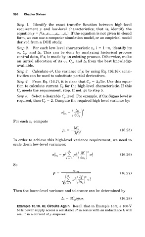
Step 3. Calculate , the variance of y, by using Eq. (16.16); sensi-
2
tivities can be used to substitute partial derivatives.
Step 4. From Eq. (16.7), it is clear that C p 0 /3 . Use this equa-
tion to calculate current C p for the high-level characteristic. If this
C p meets the requirement, stop. If not, go to step 5.
Step 5. Select a desirable C p level. For example, if Six Sigma level is
required, then C p 2. Compute the required high level variance by:

2
0
req 2
3C p
For each x i , compute
"C i
p i (16.25)
2
("f) i
In order to achieve this high-level variance requirement, we need to
scale down low-level variances:
n 2

∂f
2
2
req p 2
p i i 2 (16.26)
i 1 ∂x i
So
req
p (16.27)
i 1 ∂x i 2
n

∂f
2

2
p i
i
Then the lower-level variance and tolerance can be determined by
(16.28)
i 3C p pp i i
Example 16.10. RL Circuits Again Recall that in Example 16.9, a 100-V
f-Hz power supply across a resistance R in series with an inductance L will
result in a current of y amperes: