Page 632 - Design for Six Sigma a Roadmap for Product Development

Tolerance Design 585

16.3.3 Nonlinear statistical tolerance
If the transfer function equation between high-level requirement y and
low-level characteristics x 1 ,x 2 ,…,x i ,…,x n , is not a linear function, then
y f(x 1 ,x 2 ,…,x i ,…,x n ) (16.15)

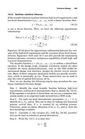
is not a linear function. Then, we have the following approximate
relationship:

∂f
∂f
∂f
Var(y) 2 1 2 2 ... 2 i 2
2
2
2
∂x 1 ∂x 2 ∂x i

∂f
... 2 n 2 (16.16)
∂x n
Equation (16.16) gives the approximate relationship between the vari-
ance of the high-level requirement and the variances of low-level charac-
teristics. Equations (16.6) and (16.7) can still provide the relationship
between tolerance, variances, and process capabilities of both high- and
low-level characteristics.
The transfer function y f(x 1 ,x 2 ,…,x i ,…,x n ) is seldom a closed-form
equation. In the design stage, computer simulation models are often
available for many products/processes, such as the FEA model for
mechanical design and electronic designs for electric circuit simula-
tors. Many of these computer simulation models can provide sensitiv-
ities, which is essentially y/ x i . These sensitivities can be used to
play the roles of partial derivatives, ∂f/∂x i .
Here we can develop the following step-by-step procedure for non-
linear statistical tolerance design:

Step 1. Identify the exact transfer function between high-level
requirement y and low-level characteristics; that is, identify Eq. (16.15).
If the equation is not given in closed form, we can use a computer sim-
ulation model, or an empirical model derived from a DOE study.
...
Step 2. For each low-level characteristic (parameter), x i , i 1 n,
identify its i , C p , and i . This can be done by looking into historical
process control data, if x i is created by an existing process.
Otherwise, make an initial allocation of its i , C p , and i , from the
best knowledge available.
2
Step 3. Calculate , the variance of y; with Eq. (16.16), sensitivi-
ties can be used to substitute partial derivatives.
Step 4. From Eq. (16.7), it is clear that

0
C p
3