Page 629 - Design for Six Sigma a Roadmap for Product Development

582 Chapter Sixteen

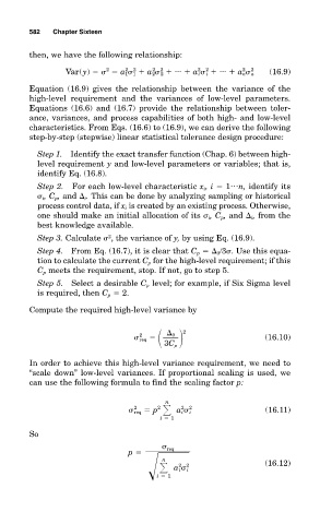
then, we have the following relationship:
2
2
2
2
2
Var(y) a 1 1 a 2 2 ... a i i ... a n n 2 (16.9)
2
2
2
Equation (16.9) gives the relationship between the variance of the
high-level requirement and the variances of low-level parameters.
Equations (16.6) and (16.7) provide the relationship between toler-
ance, variances, and process capabilities of both high- and low-level
characteristics. From Eqs. (16.6) to (16.9), we can derive the following
step-by-step (stepwise) linear statistical tolerance design procedure:
Step 1. Identify the exact transfer function (Chap. 6) between high-
level requirement y and low-level parameters or variables; that is,
identify Eq. (16.8).
Step 2. For each low-level characteristic x i , i 1 … n, identify its
i , C p , and i . This can be done by analyzing sampling or historical
process control data, if x i is created by an existing process. Otherwise,
one should make an initial allocation of its i , C p , and i , from the
best knowledge available.
Step 3. Calculate , the variance of y, by using Eq. (16.9).
2
Step 4. From Eq. (16.7), it is clear that C p 0 3 . Use this equa-
tion to calculate the current C p for the high-level requirement; if this
C p meets the requirement, stop. If not, go to step 5.
Step 5. Select a desirable C p level; for example, if Six Sigma level
is required, then C p 2.
Compute the required high-level variance by

0 2
2
req (16.10)
3C p
In order to achieve this high-level variance requirement, we need to
“scale down” low-level variances. If proportional scaling is used, we
can use the following formula to find the scaling factor p:

n
2
2
req p 2
a i i 2 (16.11)
i 1
So

req
p
i 1 2 (16.12)
n

2
a i i