Page 625 - Design for Six Sigma a Roadmap for Product Development

578 Chapter Sixteen

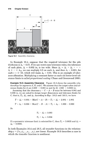
C

y = C – A – B
B
A

Figure 16.4 Assembly clearance.

In Example 16.4, suppose that the required tolerance for the pile
thickness is 0 0.01. If we use worst-case tolerance rules, the tolerance
of each plate, i 0.002 in, is too wide. Since 0 1 2 ...
i ... 10 , we can multiply 0.5 on each i , and then i 0.001, for
...
each i 1 10, which will make 0 0.01. This is an example of toler-
ance allocation. Multiplying a constant factor on each old lower-level tol-
erance limits is called proportional scaling (Chase and Greenwood 1988).
Example 16.5: Assembly Clearance Figure 16.4 shows the assembly rela-
tionships for segments A, B, and C. We assume that the target value and tol-
erance limits for A are 2.000 0.001 in and for B, 1.000 0.0001 in.
Assuming that the clearance y C A B must be between 0.001 and
0.006 in, we are asked to design target dimensions and tolerance limits for
C, that is, T C , ′ C , and C . According to Eqs. (16.2) and (16.3), we have

T ′ 0 0.001 Min(C A B) T C ′ C 2.001 1.001
T 0 0.006 Max(C B A) T C C 1.999 0.999
So

T C ′ C 3.003
T C C 3.004

If a symmetric tolerance limit is selected for C, then T C 3.0035 and ′ C
C 0.0005.

In both Examples 16.4 and 16.5, all transfer functions in the relation-
ship y f(x 1 ,x 2 ,…,x i ,…,x n ), are linear. Example 16.6 describes a case in
which the transfer function is nonlinear.