Page 627 - Design for Six Sigma a Roadmap for Product Development

580 Chapter Sixteen

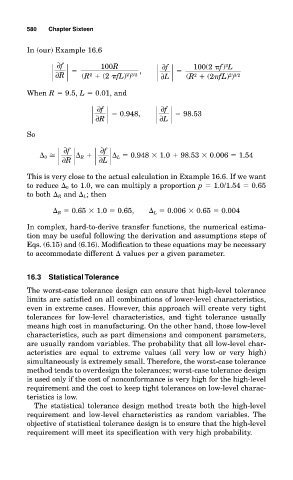
In (our) Example 16.6
∂f
,
100(2 f) L
100R
2
∂f

∂R
2 3/2
(R (2 fL) )
2
2
(R (2 fL) )
2 3/2
∂L
When R 9.5, L 0.01, and
0.948, 98.53
∂f
∂f

∂R
∂L
So

∂f
∂f
0 R L 0.948
1.0 98.53
0.006 1.54
∂R
∂L
This is very close to the actual calculation in Example 16.6. If we want
to reduce 0 to 1.0, we can multiply a proportion p 1.0/1.54 0.65
to both R and L ; then
R 0.65
1.0 0.65, L 0.006
0.65 0.004
In complex, hard-to-derive transfer functions, the numerical estima-
tion may be useful following the derivation and assumptions steps of
Eqs. (6.15) and (6.16). Modification to these equations may be necessary
to accommodate different values per a given parameter.
16.3 Statistical Tolerance
The worst-case tolerance design can ensure that high-level tolerance
limits are satisfied on all combinations of lower-level characteristics,
even in extreme cases. However, this approach will create very tight
tolerances for low-level characteristics, and tight tolerance usually
means high cost in manufacturing. On the other hand, those low-level
characteristics, such as part dimensions and component parameters,
are usually random variables. The probability that all low-level char-
acteristics are equal to extreme values (all very low or very high)
simultaneously is extremely small. Therefore, the worst-case tolerance
method tends to overdesign the tolerances; worst-case tolerance design
is used only if the cost of nonconformance is very high for the high-level
requirement and the cost to keep tight tolerances on low-level charac-
teristics is low.
The statistical tolerance design method treats both the high-level
requirement and low-level characteristics as random variables. The
objective of statistical tolerance design is to ensure that the high-level
requirement will meet its specification with very high probability.