Page 636 - Design for Six Sigma a Roadmap for Product Development

Tolerance Design 589

n
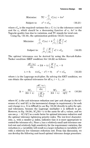
Minimize: TC
C i ( i ) k 2
i 1
2
2
Subject to: req (16.21)
2
where req is the required variance for y. C i ( i ) is the tolerance control
cost for x i , which should be a decreasing function of i . k is the
2
Taguchi quality loss due to variation, and TC stands for total cost.
Using Eq. (16.16), the optimization problem (16.21) becomes
n n ∂f 2

Minimize:
C i ( i ) k
i 2
i 1 i 1 ∂x i
n ∂f 2
2
2

Subject to:
i req (16.22)
i 1 ∂x i
The optimal tolerances can be derived by using the Karush-Kuhn-
Tucker condition (KKT condition) for (16.22) as follows:

dC i ( i ) ∂f 2
2(k !) i 0
d i ∂x i
2
2
2
2
! 0; !( req ) 0; req (16.23)
where ! is the Lagrange multiplier. By solving the KKT condition, we
can obtain the optimal tolerances for all x i , i 1,...,n:
dC ( )

i
i
d i
3C p 3C p "C i
i i (16.24)

2(k !) ∂f 2 2(k !) ("f) i 2

∂x i
where "C i is the unit tolerance reduction cost (per unit change in the tol-
erance of x i ) and ("f) i is the incremental change in requirement y for each
unit change in x i . It is difficult to use Eq. (16.24) directly to solve for opti-
mal tolerances, because the Lagrange multiplier ! is difficult to get.
However, in Eq. (16.24), 3C p /2(k !) is the same for all x i values, and we
can use p i "C i /("f) as a scale factor for optimal tolerance reduction and
2
i
the optimal tolerance tightening priority index. The low-level character-
istic, x i , with a smaller p i index, indicates that it is more appropriate to
control the tolerance of x i . Since x i has a relatively small unit tolerance con-
trol cost and relatively high sensitivity for the requirement variation, the
reduction in x i variability will result in a larger reduction in variability of Y
with a relatively low tolerance reduction cost. From this discussion, we
can develop the following cost-based optimal tolerance design procedure: