Page 107 - Distillation theory

P1: FCH/FFX P2: FCH/FFX QC: FCH/FFX T1: FCH
0521832772c04 CB644-Petlyuk-v1 June 11, 2004 17:49

4.2 Essence of Reversible Distillation Process and Its Peculiarities 81

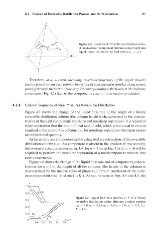
2

x t x t rev
rev
Figure 4.2. Location of reversible section trajectories
D x F y F x B x of an ideal four-component mixture at sharp split and
liquid–vapor tie-line of the feed point (x F → y F ).
1 4

3
Therefore, at α i = const, the sharp reversible trajectory of the upper (lower)
section goes from the feed point to hyperface of concentration simplex along secant,
passing through the vertex of the simplex corresponding to the heaviest (the lightest)
component (Fig. 4.2) (i.e., to the components absent in the section products).

4.2.4. Column Sequence of Ideal Mixtures Reversible Distillation
Figure 4.3 shows the change of the liquid flow rate at the height of a binary
reversible distillation column (the column height is characterized by the concen-
tration of the light component) for sharp and nonsharp separation. It is typical of
sharp separation that the input of heat and of cold, which is not equal to zero, is
required at the ends of the column and, for nonsharp separation, this input makes
an infinitesimal quantity.
As far as only one component can be exhausted in each section of the reversible
distillation column (i.e., this component is absent in the product of this section),
the system of columns shown in Fig. 4.4 (for n = 3) or in Fig. 4.5 (for n = 4) will be
required to perform the complete separation of a multicomponent mixture into
pure components.
Figure 4.6 shows the change of the liquid flow rate and of components concen-
trations for n = 3 at the height of all the columns (the height of the columns is
characterized by the inverse value of phase equilibrium coefficient of the refer-
ence component (the third one) 1/K 3 ). As can be seen in Figs. 4.4 and 4.5, the

x 1
10
.
η η
0.8 η 2 1
3
Figure 4.3. Liquid flow rate profiles L/F of a binary
0.6
reversible distillation under different product purities
(η 1 = 1.0,η 2 = 0.95,η 3 = 0.9; α = 2.0, x F = 0.5, L F /
0.4
F = 1.0).
0.2 η 3
η η 1
0 2 L/F
0.4 0.6 1.2 1.6 2.0