Page 210 - Distributed model predictive control for plant-wide systems

184 Distributed Model Predictive Control for Plant-Wide Systems

and by Lemma 8.3, we have
N−1
∑ ‖ f (N − 1)
‖
(‖x (k + s|k)‖ − ‖̂ x (k + s|k)‖ ) ≤ (8.38)
P
‖ ‖P 2
s=1
Using (8.36)–(8.38) in (8.35) then yields
( )
(N − 1) 1 1
V(k)− V(k − 1) < −1 + + + (8.39)
2 2
which, in view of (8.34), implies that V(k) − V(k − 1) < 0. Thus, for any k ≥ 0, if
x(k)∈ X∖Ω( ), there is a constant ∈ (0, ∞) such that V(k) ≤ V(k − 1) − . It then follows
′
′
that there exists a finite time k such that x(k ) ∈Ω( ). This concludes the proof.
We have now established the feasibility the DMPC and the stability of the resulting
closed-loop system. That is, if an initially feasible solution could be found, subsequent
feasibility of the algorithm is guaranteed at every update, and the resulting closed-loop system
is asymptotically stable at the origin.

8.5 Example
8.5.1 The System

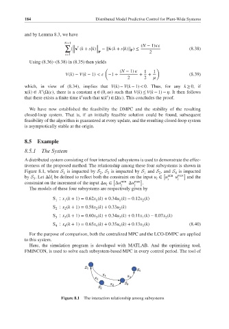
A distributed system consisting of four interacted subsystems is used to demonstrate the effec-
tiveness of the proposed method. The relationship among these four subsystems is shown in
Figure 8.1, where S is impacted by S , S is impacted by S and S , and S is impacted
1
2
3
1
4
2 [
by S .Let ΔU be defined to reflect both the constraint on the input u ∈ u min u max ] and the
i
3
i
[ min max ] i i
constraint on the increment of the input Δu ∈ Δu i Δu i .
i
The models of these four subsystems are respectively given by
S ∶ x (k + 1)= 0.62x (k)+ 0.34u (k)− 0.12x (k)
1
1
1
1
2
S ∶ x (k + 1)= 0.58x (k)+ 0.33u (k)
2
2
2
2
S ∶ x (k + 1)= 0.60x (k)+ 0.34u (k)+ 0.11x (k)− 0.07x (k)
3
3
3
1
3
2
S ∶ x (k + 1)= 0.65x (k)+ 0.35u (k)+ 0.13x (k) (8.40)
4
3
4
4
4
For the purpose of comparison, both the centralized MPC and the LCO-DMPC are applied
to this system.
Here, the simulation program is developed with MATLAB. And the optimizing tool,
FMINCON, is used to solve each subsystem-based MPC in every control period. The tool of
1
4
x 1
x 3
x 2
3
x 2
2
Figure 8.1 The interaction relationship among subsystems