Page 229 - Distributed model predictive control for plant-wide systems

Cooperative Distributed Predictive Control with Constraints 203

S ∶ x (k + 1)= 0.681x (k)+ 0.415u (k)
5 5 5 5
+ 0.068x (k)+ 0.068x (k)+ 0.068x (k)
4 6 7
S ∶ x (k + 1)= 0.548x (k)+ 0.376u (k)
6
6
6
6
+ 0.055x (k)+ 0.055x (k)
7
5
S ∶ x (k + 1)= 0.716x (k)+ 0.425u (k)
7
7
7
7
+ 0.018x (k)+ 0.018x (k)+ 0.018x (k)
3
2
1
+ 0.018x (k)+ 0.018x (k)+ 0.018x (k)
6
4
5
For the purpose of comparison, the centralized MPC, local cost optimization based MPC,
and the C-DMPC are all applied to this system.
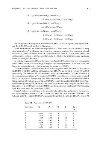
Some parameters of the controllers in proposed C-DMPC are shown in Table 9.2. Among
these parameters, P is obtained by solving the Lyapunov function. The eigenvalue of each
i
closed-loop system under the feedback control shown in Table 9.2 is 0.5. Set = 0.15, and
set the control horizon of all the controllers to be N = 10. Set the initial presumed inputs and
states, at time k = 0, be zeros.
0
In both the centralized MPC and the subsystem-based MPCs of the local cost optimization
based DMPC, the dual mode strategy is adopted, and set the parameters, the initial states, and
the initial presumed inputs to be the same as those used in C-DMPC.
The state responses and the inputs of the closed-loop system under the control of the central-
ized MPC, C-DMPC, and local optimization based DMPC are shown in Figures 9.3 and 9.4,
respectively. The shape of the state response curves under the control C-DMPC is similar to
those under the centralized MPC. Under the C-DMPC control design, when set-point changed,
there is no significant overshooting, but some fluctuations exist in the trajectories of states of
the interacting subsystems. Under the LCO-DMPC control design, the states of all subsystems
could converge to set-point, but there exists much larger overshooting comparing to those under
the control of C-DMPC and centralized MPC, and there are larger amplitude in the fluctuating
state than those under the control of C-DMPC.
Figure 9.5 shows the difference of the absolute value of the state and inputs of each subsys-
tem between under the control of LCO-DMPC and under the control of centralized MPC, and
between under the control of C-DMPC and under the control of centralized DMPC. Figure 9.6

Table 9.2 Parameters of C-DMPC

Subsystem K i P i Q i R i Δu i,U
Δu
i,L
S −0.44 5.38 4 0.2 ± 1
1
S −0.34 5.36 4 0.2 ± 1
2
S −0.37 5.37 4 0.2 ± 1
3
S 4 −0.52 5.40 4 0.2 ± 1
S 5 −0.68 5.46 4 0.2 ± 1
S 6 −0.37 5.37 4 0.2 ± 1
S 7 −0.76 5.49 4 0.2 ± 1