Page 241 - Distributed model predictive control for plant-wide systems

Networked Distributed Predictive Control with Inputs and Information Structure Constraints 215

Set each presumed state sequence ̂ x to be the remainder of the sequence predicted at time
j,i
instant k − 1, concatenated with the closed-loop response under the state feedback control
p
̂ u (k + s − 1|k)= K x (k + N − 1|k − 1), that is
j,i
j j,i
p
̂ x (k + s − 1|k)= x (k + s − 1|k − 1), s = 1, 2, … , N (10.8)
j,i
j,i
p
and ̂ x (k + N |k)= x (k + N |k − 1) is calculated by substituting ̂ u (k + N − 1|k) into (10.5)
j,i
j,i
j,i
based on the presumed state sequence obtained at time k − 1.
In addition, a decoupled terminal-state constraint will be included in each subsystem-based
MPC, which guarantees that the terminal controllers are stabilizing inside a terminal set. To
define this terminal state set, we need to make an assumption and establish a technical lemma.
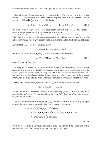
Assumption 10.2 The block-diagonal matrix
A = block-diag{A , A , … , A }
d d1 d2 dm
and the off-diagonal matrix A = A − A satisfy the following inequality:
o c d
T
T
T
A PA + A PA + A PA < Q∕2 (10.9)
̂
o
d
o
o
o
d
T
̂
where Q = Q + K RK > 0.
It, along with Assumption 10.1, helps with the design of the terminal set. This assumption
quantifies how much strengthening the coupling among subsystems is sufficient so that the
overall system can be stabilized by the proposed DMPC here. This assumption is not necessary,
and some systems that do not satisfy this assumption may also be stabilized by the proposed
DMPC, and the more relaxing condition is still remaining to be designed in the future work.
Lemma 10.1 Under Assumptions 10.1 and 10.2, for any positive scalar c the set
Ω(c)={x ∈ ℝ n x ∶ ‖x‖ ≤ c}
P
is a positive invariant region of attraction for the closed-loop system x(k + 1)= A x(k). Addi-
c
tionally, there exists a small enough positive scalar such that Ω( ) is in the feasible input set
U ∈ ℝ n u for all x ∈Ω( ).
2
Proof. Consider the function V(k)= ‖x (k)‖ . The time difference of V(k) along the trajec-
P
tories of the closed-loop system x(k + 1) = A x(k) can be evaluated as
c
T
T
T
ΔV(k)= x (k)A PA x(k)− x (k)Px(k)
c
c
T
T
T
T
T
= x (k)(A PA − P + A PA + A PA + A PA )x(k)
d d o o o d d o
T
1 T
≤ −x (k)Qx(k)+ x (k)Qx(k)
̂
̂
2
≤ 0 (10.10)
which holds for all x(k) ∈Ω(c)\{0}. This implies that all trajectories of the closed-loop system
that start inside Ω(c) will remain inside and converge to the origin.