Page 238 - Distributed model predictive control for plant-wide systems
P. 238
212                           Distributed Model Predictive Control for Plant-Wide Systems


             The control objective is to stabilize the overall system S in a DMPC framework. And the
           performance of entire closed-loop system should be as close as that under the control of cen-
           tralized MPC and the communication cost should not be too high.
             The coordination strategy as proposed in Chapter 7 is a preferable method to tradeoff
           between the communication burden and the global performance. However, the DMPC under
           this coordination strategy does not take the constraints into consideration. A noniterative
           stabilizing DMPC that takes constraints into consideration remains to be developed either
           under this coordination strategy or some other coordination strategies reviewed earlier. The
           objective of this chapter is to develop such a DMPC design.


           10.3   Constrained N-DMPC
           10.3.1   Formulation

           In this section, m separate optimal control problems, one for each subsystem, and the N-DMPC
           algorithm are defined. In each of these optimal control problems, the same constant prediction
           horizon N, N ≥ 1, is used. The resulting m separate subsystem-based MPC laws are updated
           synchronously. At each update, every subsystem-based MPC optimizes only over its own
           predicted open-loop control, given its impacted region’s current states, and their upstream
           subsystems’ estimated inputs and states.
             To proceed, we need the following assumption:


           Assumption 10.1  For every subsystem S , ∀i ∈ P, there exists a state feedback u =
                                               i
                                                                                  i,k
           K x   such that the closed-loop system x(k + 1) = A x(k) is asymptotically stable, where
             i i,k                                     c
           A = A + BK and K = block-diag{K , K , … , K }.
             c                          1   2     m
             This assumption is usually used in the design of stabilizing DMPC [26, 34]. It presumes
           that each subsystem is able to be stabilized by a decentralized control K x , i ∈ P.
                                                                     i i
             We also define the necessary notation in Table 10.1.
             As the state evolution of the downstream subsystems of S is affected by the optimal control
                                                           j
           decision of S , the performance of these downstream subsystems may be affected negatively
                      i
           by the control decision of S . Thus, in the ICO-DMPC, each subsystem-based MPC takes into
                                 i
           account the cost functions of its downstream subsystems. More specifically, the performance
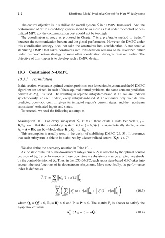
           index is defined as
                               ∑  ‖ p          2
                         J (k)=               ‖
                          i       ‖x (k + N |k)‖
                                  ‖ j,i
                                              ‖P j
                               j∈P i
                                    (                                 )
                                 N−1
                                 ∑    ∑  ‖ p         2   ‖ p         2
                                                                   ‖
                                                    ‖
                               +         ‖x (k + s|k)‖  + ‖u (k + s|k)‖          (10.3)
                                         ‖ j,i      ‖Q j  ‖ i      ‖R i
                                  s=0  j∈P i
                                   T
                                                 T
                       T
           where Q = Q > 0, R = R > 0 and P = P > 0. The matrix P is chosen to satisfy the
                  i    i      i    i         i   i               i
           Lyapunov equation
                                         T
                                                       ̂
                                        A P A − P =−Q   i                        (10.4)
                                         di i
                                              di
                                                  i

