Page 243 - Distributed model predictive control for plant-wide systems

Networked Distributed Predictive Control with Inputs and Information Structure Constraints 217

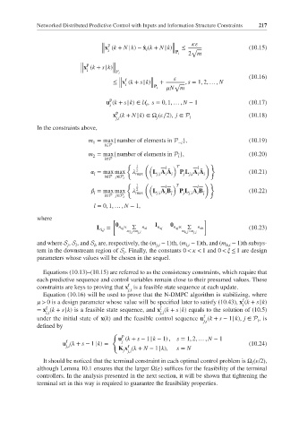
‖ p ‖ (10.15)
‖x (k + N |k) − ̂ x (k + N |k)‖ ≤ √
‖ i i ‖P i
2 m
‖ p ‖
‖x (k + s|k)‖
‖ i ‖P i
(10.16)

‖ f
‖
≤ ‖x (k + s|k)‖ + √ , s = 1, 2, … , N
i
N m
‖ ‖P i
p
u (k + s|k)∈ U , s = 0, 1, … , N − 1 (10.17)
i i
p
x (k + N |k)∈Ω ( ∕2), j ∈ P (10.18)
j,i j i
In the constraints above,
m =max{number of elements in P }, (10.19)
−i
1
i∈P
}, (10.20)
2
m =max{number of elements in P̃ i
i∈P
{ ( )}
1 ( l ) T l
̃
̃
=max max 2 L A A P L A A (10.21)
l max j,i i i j j,i i i
i∈P j∈P i
{ ( )}
1 ( l ) T l
2
=max max max L A B i P L A B i (10.22)
i
j,i
l
j j,i
i
i∈P j∈P i
l = 0, 1, … , N − 1,
where [ ]
∑ I ∑
L = n xj × n xl n xj n xj × n xh (10.23)
i,j
m l,i <m j,i m h,i >m j,i
and where S , S , and S are, respectively, the (m − 1)th, (m − 1)th, and (m − 1)th subsys-
j l h j,i l,i h,i
tem in the downstream region of S . Finally, the constants 0 < < 1 and 0 < ≤ 1 are design
i
parameters whose values will be chosen in the sequel.
Equations (10.13)–(10.15) are referred to as the consistency constraints, which require that
each predictive sequence and control variables remain close to their presumed values. These
f
constraints are keys to proving that x is a feasible state sequence at each update.
j,i
Equation (10.16) will be used to prove that the N-DMPC algorithm is stabilizing, where
f
> 0 is a design parameter whose value will be specified later to satisfy (10.43), x (k + s|k)
i
f
f
= x (k + s|k) is a feasible state sequence, and x (k + s|k) equals to the solution of (10.5)
i,i j,i
f
under the initial state of x(k) and the feasible control sequence u (k + s − 1|k), j ∈ P ,is
j,i i
defined by
{
p
u (k + s − 1|k − 1) , s = 1, 2, … , N − 1
f
j
u (k + s − 1|k)= (10.24)
j,i f
K x (k + N − 1|k), s = N
j j,i
It should be noticed that the terminal constraint in each optimal control problem is Ω ( /2),
i
although Lemma 10.1 ensures that the larger Ω( ) suffices for the feasibility of the terminal
controllers. In the analysis presented in the next section, it will be shown that tightening the
terminal set in this way is required to guarantee the feasibility properties.