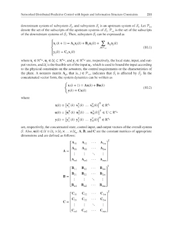
Page 237 - Distributed model predictive control for plant-wide systems

Networked Distributed Predictive Control with Inputs and Information Structure Constraints 211

downstream system of subsystem S , and subsystem S is an upstream system of S .Let P +i
j
i
j
denote the set of the subscripts of the upstream systems of S , P −i is the set of the subscripts
i
of the downstream systems of S . Then, subsystem S can be expressed as
i i
∑
⎧
x (k + 1) = A x (k)+ B u (k)+ A x (k)
i
ii i
ij j
ii i
⎪
j∈P +i (10.1)
⎨
⎪y (k)= C x (k)
i ii i
⎩
where x ∈ ℝ , u ∈ U ⊂ ℝ , and y ∈ ℝ n yi are, respectively, the local state, input, and out-
n ui
n xi
i i i i
put vectors, and U is the feasible set of the input u , which is used to bound the input according
i i
to the physical constraints on the actuators, the control requirements or the characteristics of
the plant. A nonzero matrix A , that is, j ∈ P , indicates that S is affected by S .Inthe
ij +i i j
concatenated vector form, the system dynamics can be written as
{
x (k + 1) = Ax(k)+ Bu(k)
(10.2)
y(k)= Cx(k)
where
[ T T T ] T
x(k)= x (k) x (k)… x (k) ∈ R n x
1 2 m
[ T T T ] T
u(k)= u (k) u (k)… u (k) ∈ U ⊂ R n u
m
1 2
[ T T ] T
T
y(k)= y (k) y (k)… y (k) ∈ R n y
m
1 2
are, respectively, the concatenated state, control input, and output vectors of the overall system
S.Also, u(k)∈ U = U × U ×…× U . A, B, and C are the constant matrices of appropriate
1 2 m
dimensions and are defined as follows:
T
A A ··· A
⎡ 11 12 1m⎤
A 21 A 22 ··· A 2m
⎢ ⎥
A = ⎢ ⎥
⎢ ⋮ ⋮ ⋱ ⋮ ⎥
⎢ ⎥
⎣A A ··· A ⎦
m1 m2 mm
T
B B ··· B
⎡ 11 12 1m⎤
B 21 B 22 ··· B 2m
⎢ ⎥
B = ⎢ ⎥
⎢ ⋮ ⋮ ⋱ ⋮ ⎥
⎢ ⎥
⎣B B ··· B ⎦
m1 m2 mm
T
C C ··· C
⎡ 11 12 1m⎤
C 21 C 22 ··· C 2m
⎢ ⎥
C = ⎢ ⎥
⎢ ⋮ ⋮ ⋱ ⋮ ⎥
⎢ ⎥
⎣C C ··· C ⎦
m1 m2 mm