Page 256 - Distributed model predictive control for plant-wide systems

230 Distributed Model Predictive Control for Plant-Wide Systems

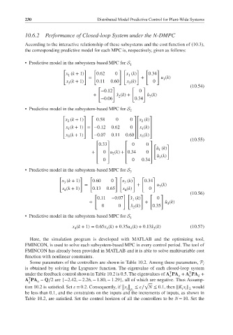
10.6.2 Performance of Closed-loop System under the N-DMPC

According to the interactive relationship of these subsystems and the cost function of (10.3),
the corresponding predictive model for each MPC is, respectively, given as follows:

• Predictive model in the subsystem-based MPC for S 1
[ ] [ ][ ] [ ]
x (k + 1) 0.62 0 x (k) 0.34
1
1
= + u (k)
1
x (k + 1) 0.11 0.60 x (k) 0
3 3
(10.54)
[ ] [ ]
−0.12 0
+ ̂ x (k)+ ̂ u (k)
2
3
−0.06 0.34
• Predictive model in the subsystem-based MPC for S 2
⎡ 0.58 0
⎡x (k + 1)⎤ 0 ⎤ ⎡x (k)⎤
2 2
⎢ ⎥ ⎢ ⎥ ⎢ ⎥
x (k + 1) = −0.12 0.62 0 x (k)
⎢ 1 ⎥ ⎢ ⎥ ⎢ 1 ⎥
⎢ x (k + 1) ⎥ ⎢ −0.07 0.11 0.60 ⎥ ⎢ x (k) ⎥
⎣ 3 ⎦ ⎣ ⎦ ⎣ 3 ⎦
(10.55)
⎡0.33⎤ ⎡ 0 0 ⎤ [ ]
⎥ ̂u (k)
⎢ ⎥ ⎢ 1
+ 0 u (k)+ 0.34 0
⎢ ⎥ 2 ⎢ ⎥
̂ u (k)
⎢ 0 ⎥ ⎢ 0 0.34 ⎥ 3
⎣ ⎦ ⎣ ⎦
• Predictive model in the subsystem-based MPC for S 3
[ ] [ ][ ] [ ]
x (k + 1) 0.60 0 x (k) 0.34
3
3
= + u (k)
3
x (k + 1) 0.13 0.65 x (k) 0
4 4
(10.56)
[ ][ ] [ ]
0.11 −0.07 ̂ x (k) 0
1
+ + ̂ u (k)
4
0 0 ̂ x (k) 0.35
2
• Predictive model in the subsystem-based MPC for S 4
x (k + 1)= 0.65x (k)+ 0.35u (k)+ 0.13̂x (k) (10.57)
4 4 4 3
Here, the simulation program is developed with MATLAB and the optimizing tool,
FMINCON, is used to solve each subsystem-based MPC in every control period. The tool of
FMINCON has already been provided in MATLAB and it is able to solve multivariable cost
function with nonlinear constraints.
Some parameters of the controllers are shown in Table 10.2. Among these parameters, P
i
is obtained by solving the Lyapunov function. The eigenvalue of each closed-loop system
T
T
under the feedback control shown in Table 10.2 is 0.5. The eigenvalues of A PA + A PA +
o
o
o
d
T
A PA − Q∕2are {−2.42, − 2.26, − 1.80, − 1.29}, all of which are negative. Thus Assump-
o
d √
tion 10.2 is satisfied. Set = 0.2. Consequently, if x ≤ ∕ N ≤ 0.1, then ‖K x ‖ would
‖ ‖
i i 2
‖ i‖p i
be less than 0.1, and the constraints on the inputs and the increments of inputs, as shown in
Table 10.2, are satisfied. Set the control horizon of all the controllers to be N = 10. Set the