Page 252 - Distributed model predictive control for plant-wide systems

226 Distributed Model Predictive Control for Plant-Wide Systems

n
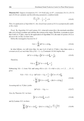
Theorem 10.2 Suppose Assumptions 10.1–10.3 hold, x(k )∈ ℝ x , constraints (10.13)–(10.15)
0
and (10.16) are satisfied, and the following parametric condition holds:
(N − 1) 1 1
− + < 0 (10.43)
2 2
Then, by application of Algorithm 8.1, the closed-loop system of (8.2) is asymptotically stable
at the origin.

Proof. By Algorithm 10.1 and Lemma 10.1, when x(k) enters Ω( ), the terminal controllers
take over to keep it in there and stabilize the system at the origin. Therefore, it remains to show
that if x(0)∈ X∖Ω( ), then by the application of Algorithm 10.1, the state of system (10.2) is
driven to the set Ω( ) in finite time.
Define the nonnegative function for S

N
∑ p
V(k)= ‖x (k + s|k)‖ P (10.44)
s=1
In what follows, we will show that, for any k ≥ 0, if x(k)∈ X∖Ω( ), then there exists a
constant ∈ (0, ∞) such that V(k) ≤ V(k − 1) − . Constraint (10.16) implies that

‖ f
p
‖
‖x (k + s|k)‖ ≤ ‖x (k + s|k)‖ + (10.45)
P
‖ ‖P N
Therefore,
N
∑ ‖ f
‖
V(k) ≤ ‖x (k + s|k)‖ +
‖ ‖P
s=1
p
Subtracting V(k − 1) from V(k) and using x (k + s|k − 1)= ̂ x(k + s|k), s = 1, 2, … , N − 1,
gives
p
V(k)− V(k − 1) ≤ −‖x (k|k − 1)‖ + ‖ f ‖
P + ‖x (k + N |k)‖
‖ ‖P
(10.46)
N−1 ( )
∑ ‖ f ‖
+ ‖x (k + s|k)‖ − ‖̂ x (k + s|k)‖ P
‖ ‖P
s=1
Assuming x(k)∈ X∖Ω( ) yields
p
‖x (k|k − 1)‖ > (10.47)
P
Also, by Theorem 10.1 we have
‖ f ‖
‖x (k + N |k)‖ ≤ ∕2 (10.48)
‖ ‖P
and by Lemma 10.3, we have
N−1 ( )
∑ (N − 1)
‖ f ‖
‖x (k + s|k)‖ − ‖̂ x (k + s|k)‖ P ≤ (10.49)
‖ ‖P 2
s=1